Tag: pattern

There are some quite well known procedural content generation algorithms out there: Voronoi, Perlin noise, simplex noise, L-systems, reaction-diffusion systems like Turing pattern, which I’ve presented in my earlier blog post.The specifics of these algorithms are that either generates a large amount of content for a small investment of input data, or one that adds structure to random noise.

Generally speaking they are categorized by what they generate (map vs sequence generation) and also by the mindset behind their use. This time we’ll discuss the Worley noise pattern, which can be included into the generative map creation category. This means we need a grid system for the representation and visualization of points scattered randomly in 3D or 2D space.

In it’s visual appearance is almost like a Voronoi diagram, only it’s not as famous like it’s counterpart. Even Wikipedia discuss it very briefly. Worley noise in it’s essence is a noise generation pattern, which means by multiplication/addition of different octaves of the same noise pattern we can produce a variety and completely different outputs. This is the fun part of working with generative patterns.

Now, after we gain a little theoretical introduction let’s get started with the basics, and try to dissect how can we reproduce those organic shapes and textures found in every living being in nature. (In parentheses being said, in many graphic simulations and parametric applications dealing with textural visualizations this shapes can be found). As a last side note before we go into the technical details, my intention was to implement the algorithm in Javascript mainly because i wished to be accessible by as many users as possible, and at the same time i was curious how far can i stress the limit of the modern web browsers. This is an experiment based 100% on CPU, so WebGL was out of scope, only because i was not playing with this technology until now, but i considering to implement on GPU in a shorter or longer future.

Feature points

The basic idea is to spread randomly varying number in space and calculate the distance to these point from every possible location of space. As a complement, Worley suggest to assign to each feature point an unique ID number. This number can be used to generate surface with colored areas or crocodile like textures, cityblock diagrams etc. depending on the algorithm, or coloring function implemented.

The noise function simply computes a single value for every location in space. We can then use that value in literally thousands of interesting ways, such as perturbing an existing pattern spatially, mapping directly to a density or color or adding multiple scale of noise to make a fractal combination. While there are infinite number of possible functions which provide an infinite number of outputs, noise’s random behavior gives a much more interesting appearance  then simple gradients for example.

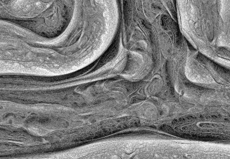
By spreading  feature points randomly through the 3D space we build a scalar function based on the distribution of the points near the sample location. Because an image worth a thousand of words the picture below describes a space with feature points scattered across the plane.

For a position on the plane (marked with x in the picture above) there is always a closest feature point, a second closest, a third and so on. The algorithm is searching for such feature points, return  their relative distance to the target point, their position and their unique ID number.

Another key component of the algorithm is the demarcation line which is supposed to be integer in every plane. Each squares (cubes in 3D) are positioned so that their identification numbers can be expressed with some integer values. Let’s suppose we want to obtain the distance to the two feature point closest to the (3.6, 5.7) we start by looking at the integer squares (3, 5) and compare it’s feature points to each other.  It’s obvius that the two feature points in that square aren’t the two closest. One of them is, but the second closest belongs to the integer square (3, 6).

It’s possible that some feature points are not inside the square where the target point is placed, in this case we extend our analysis to the adjacent squares. We could just test all 26 immediate neighboring cubes, but by checking the closest distance we’ve computed so far (our tentative n-th closest feature distance) we can throw out whole rows of cubes at once by deciding when no point in the neighbor cube could possibly contribute to our list. We don’t know yet what points are in the adjacent cubes marked by “?,” but if we examine a circle of radius F1, we can see that it’s possible that the cubes labeled A, B, and C might contribute a closer feature point, so we have to check them. As resulted from the image below, it’s mostly possible to check 6 facing neighbors of center cube (these are the closest and most likely to have a close feature point), 12 edge cube and 8 corner cubes in 3D. We could start testing more distant cubes, but it’s much more convenient to just use a high enough density to ensure that the central 27 are sufficient.

The code implementation in Javascript

For the code implementation i used html5 canvas. I’ve commented the source code, so won’t be too hard to follow for anyone. Because (as i mentioned in the beginning) my WebGL knowledge is quite minimal, for this reason i tried to optimize every single bit of code. For this reason my single option was to use web workers by separating the main core from the computationally heavy and intense pixel manipulation logic. There is a well described article on html5rocks.com about the basic principles of web workers, followed by some very neat examples regarding the implementation of them.

The main advantage of using web workers is that we can eliminate the bottlenecks caused by computational heavy threads running in the background, separating the implementation interface from the computational logic. This way we can reduce the hangouts caused by intensive calculations which may block the UI or script to handle the user interaction.

Creating a web worker is quite simple. We define the variables we want to pass to workers, and by calling an event listener using postMessage function we transfer the main tread instructions to the worker (which is running in a separate thread). Because web workers run in isolated threads, the code that they execute needs to be contained in a separate file. But before we do that, the first thing we have to do is create a new Worker object in our main page. The constructor takes the name of the worker script:

In  a separate script we’ll define wich are the variables we want to listen for. This part is responsible for the heavy weight operations. After the pixel calculations has been done, we pass over the results through the postMessage method to the main thread. This part of code looks like the following:

As a last option i’ve included the DAT.GUI lightweight graphical interface for a user interaction, where we can select different methods, colors etc. and lastly to offer the possibility for rendering with or without web workers.

Hopefully you find interesting this experiment, and if you have some remarks, comments, then please use the comments field below, or share through twitter.