Blog

Delaunay image triangulation
In this article we present a technique to triangulate source images, converting them to abstract, someway artistic images composed of tiles of triangles. This will be an attempt to explore the fields between computer technology and art.

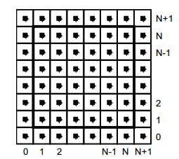
But first, what is triangulation? Simply spoken a triangulation partitions a polygon into triangles which allows, for instance, to compute the area of a polygon and execute some operations on the computed polygon surface. In other terms the triangulation might be conceived as a geometric object defined by a point set, but what differentiates the polygons from a point set is the latter does not have an interior, except if we treat the point set as a convex hull/polygon. But to think of a point set as a convex polygon, the points from the interior of the convex hull should not be ignored completely. This is what differentiates the Delaunay triangulation from the other triangulation techniques.

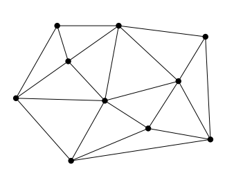
Fig.1: Point set triangulation.

Delaunay triangulation

Wikipedia has a very succinct definition of the Delaunay triangulation:

… a Delaunay triangulation (also known as a Delone triangulation) for a given set P of discrete points in a plane is a triangulation DT(P) such that no point in P is inside the circumcircle of any triangle in DT(P)

The circumcircle of a triangle is the unique circle passing through all the vertices of the triangle. This will get valuable meaning in the following. So considering that we have a set of six points we can obtain a triangulated polygon by tracing a circle around each vertex of the constructed triangle in such a manner that the circumcircle of all five triangles are empty. We also say, that the triangles satisfy the empty circle property (Fig.2).

Fig.2: All triangles satisfy the empty circle property.

After a short theoretical introduction now we want to apply this technique to a more practical but at the same time aesthetical field, concretely to transform a source image to it’s triangulated counterpart. Having the basic idea and it’s theoretical background we can start to construct the basic building blocks of the algorithm.

Above all a short notice: we use Go as programming language for the implementation. First, because it has a very clean and easy to use API, second because it can be well suited for a CLI based application, which single scope is to convert an input file to a destination object.

The algorithm

Now into the algorithm. As the basic components are triangles we define a Triangle structs, having as constituents the nodes, it’s edges and the circumcircle which describes the triangle circumference.
```
type Triangle struct {
      Nodes  []Node
      edges  []edge
      circle circle
}
```
Next we create the circumscribed circle of this triangle. The circumcircle of a triangle is the circle which has the three vertices of the triangle lying on its circumference. Once we have the circle center point we can calculate the distance between the node points and the triangle circumcircle. Then we can calculate the circle radius.

We can transpose this into the following Go code:

<br />

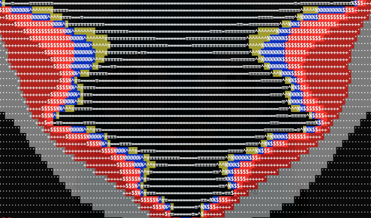
The question is how do we get the triangle points from the input image? To obtain a large triangle distribution on the image parts with more details we need somehow to analyze the image and mark the sensitive information. How do we do that? Sobel filter operator on the rescue. The Sobel operator is used in image processing to detect image edges. It’s working with an energy distribution matrix to differentiate the sensitive image informations from the less sensitive ones.

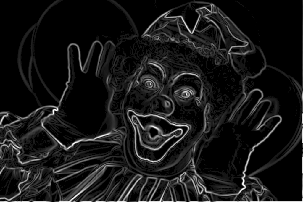
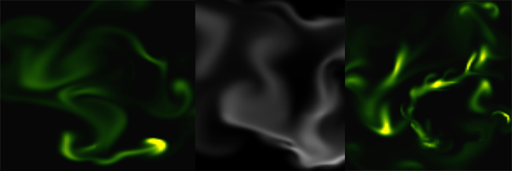
Fig.3: Sobel operator applied to the source image.

Once we obtained the sobel image we can sparse the triangle points randomly by applying some threshold value. At the end we obtain an array of randomly distributed points, but these points are more dense on the sensitive image parts, and scarce on less sensitive ones.

Having the edge points we check whether the points are inside the triangle circumcircle or not. We save the triangle edges in case they are included and carry over otherwise. Then in a loop we search for (almost) identical edges and remove them.

<br />

Now that we have the nodes, in order to construct the triangulated image, the last thing we need to do is actually to draw the lines between nodes points by applying the underlying image pixel colors. The way we can achieve this is to loop over all the nodes and connect each edge point.

<br />

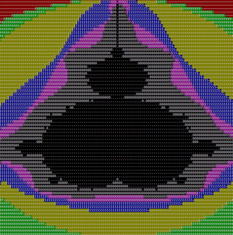
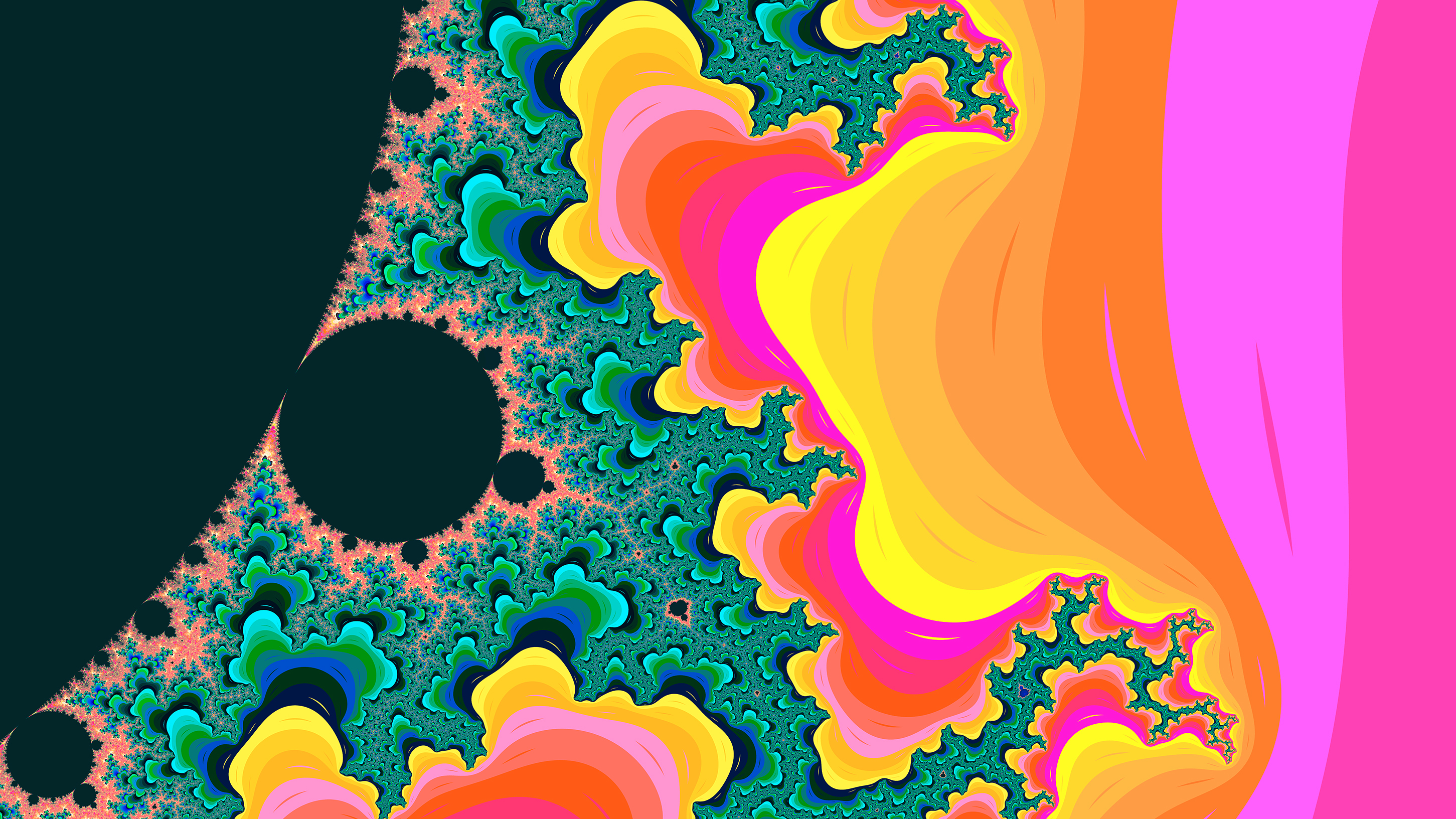
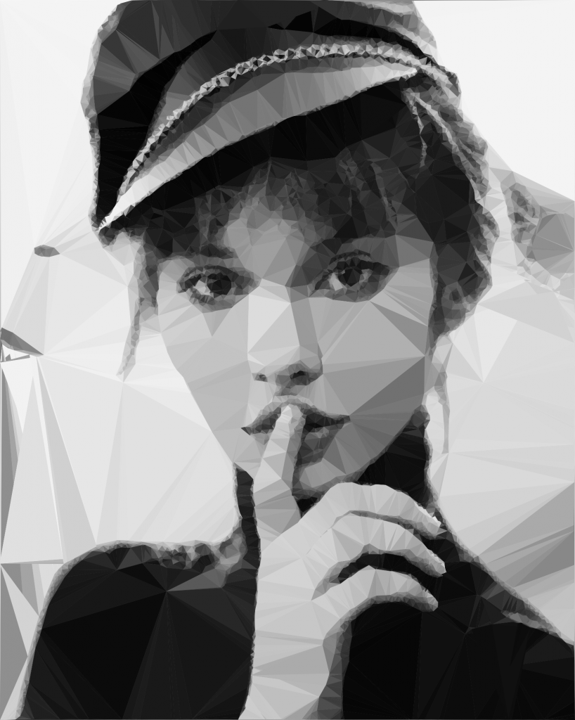
By tweaking the parameters we can obtain different kind of results. We can draw only the line strokes, we can apply different threshold values to filter out some edges, we can scale up or down the triangle sizes by defining the maximum point limit, we can export only to grayscale mode etc. The possibilities are endless.

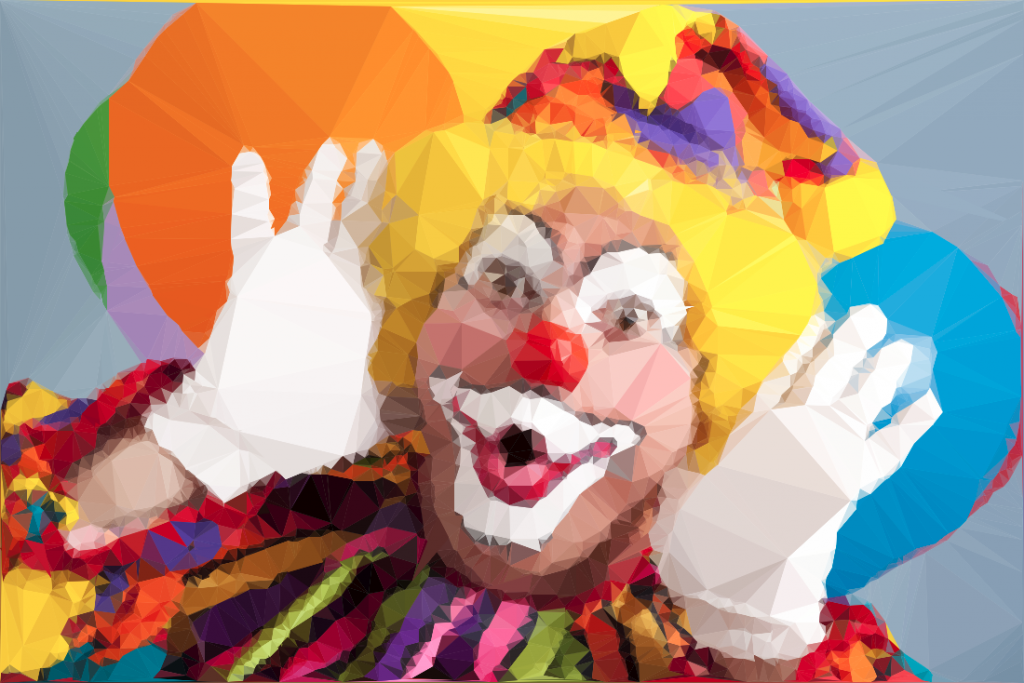
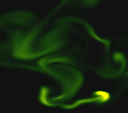
Fig.4: Triangulated image example.

Using Go interfaces to export the end result into different formats

By default the output is saved to an image file, but using interfaces, the Go way to achieve polymorphism, we can export even to a vector format. This is a nice touch considering that using a small image as input element we can export the result even to an svg file, which lately can be scaled up infinitely without image loss and consuming very low processing footprint.

The only thing we need to do is to declare an interface having a single method signature. This needs to be satisfied by each struct type implementing this method.

<br />

In our case we need two struct types, both of them implementing the same method differently. For example we could have an image struct type and an svg struct type declared in the following way:

<br />

Each of them will implement the same Draw method differently.

Expose the algorithm as an API endpoint

Having a good system architecture, coupled with Go blazing fast execution time and goroutines (another feature of the Go language to parallelize the execution) the algorithm can be exposed to an API endpoint in order to process a large amount of images and then make it accessible through a web application.

The source code can be found on my Github page:

https://github.com/esimov/triangle

I have also created an Electron/React desktop application for everyone who do not want to be bothered with the terminal commands and needs something more user friendly.

The source file can also be found on my Github account:
https://github.com/esimov/triangle-app
April 29, 2019
$ASCII terminal mandelbrot fractal renderer in Go$

ASCII terminal mandelbrot fractal renderer in Go
After the previous post about the mandelbrot renderer written in Go, this article will be related to the same topic, only this time i’ll talk about a terminal based Julia set generator written again in Go language. In fact i’ve done this experiment prior to write the mandelbrot renderer. About the implementation I’ve discussed in the last article.

The whole idea came from the motivation to create something which resembles the feeling which only a terminal based application can create (something which is close enough to the pixelart technique), but at the same time it has enough visually appealing characteristics and above all it’s dynamic.

Into the terminal fractals

(In preview the ASCII Mandelbrot generator running in terminal)

Because in the last few months i was pretty much delved into the fractals, i’ve started to create some small experiments, one of them being the code snippet below:

https://gist.github.com/esimov/970a3816dda12e4059e3.js

Which produce the following terminal output:

This was nice but i wanted to be dynamic, and not something simply put in the terminal window. So i’ve started to search for methods to refresh the terminal window periodically, ideally to refresh on each mandelbrot iteration. For this reason i’ve created some utility methods to get the terminal window width and height. And another method to flush the screen buffer periodically.
```
// Get console width
func Width() int {
	ws, err := getWinsize()

	if err != nil {
		return -1
	}

	return int(ws.Row)
}

// Get console height
func Height() int {
	ws, err := getWinsize()
	if err != nil {
		return -1
	}
	return int(ws.Col)
}

// Flush buffer and ensure that it will not overflow screen
func Flush() {
	for idx, str := range strings.Split(Screen.String(), "\n") {
		if idx > Height() {
			return
		}

		output.WriteString(str + "\n")
	}

	output.Flush()
	Screen.Reset()
}
```
It was missing another ingredient: in terminal based application we need somehow to specify the cursor position where to output the desired character, some kind of pointer to a position specified by width and height coordinate. For this i’ve created another method which move the cursor to the desired place, defined by x and y:
```
// Move cursor to given position
func MoveCursor(x int, y int) {
	fmt.Fprintf(Screen, "\033[%d;%dH", x, y)
}
```
Then we can clear the screen buffer periodically. In linux based systems to move the cursor to a specific place in terminal window we can use ANSI escape codes, like: \033[%d;%dH, where %d;%d we can replace with values obtained from the mandelbrot renderer. In the example provided in the project github repo i’m moving the terminal window cursor to the mandelbrot x and y position, after which i’m clearing the screen.

To make it more attractive i used a cheap trick to zoom in and out into the fractal and to smoothly displace the fractal position by applying sine and cosine function on x and y coordinate.
```
for {
	n += 0.045
	zoom += 0.04 * math.Sin(n)
	asciibrot.DrawFractal(zoom, math.Cos(n), math.Sin(n)/zoom*0.02, math.Sin(n), MAX_IT, true, isColor) //where math.Cos(n) and math.Sin(n) are x and y coordinates	
}
```
But there is another issue. We need to handle differently the code responsible to obtain the terminal window size in different operating systems. In linux and darwin based operating systems here is how we can get the terminal size:
```
func getWinsize() (*winsize, error) {
	ws := new(winsize)

	var _TIOCGWINSZ int64

	switch runtime.GOOS {
	case "linux":
		_TIOCGWINSZ = 0x5413
	case "darwin":
		_TIOCGWINSZ = 1074295912
	}

	r1, _, errno := syscall.Syscall(syscall.SYS_IOCTL,
		uintptr(syscall.Stdin),
		uintptr(_TIOCGWINSZ),
		uintptr(unsafe.Pointer(ws)),
	)

	if int(r1) == -1 {
		fmt.Println("Error:", os.NewSyscallError("GetWinsize", errno))
		return nil, os.NewSyscallError("GetWinsize", errno)
	}
	return ws, nil
}
```
In Windows operating system to obtain the terminal dimension is a little bit different:
```
type (
	coord struct {
		x int16
		y int16
	}

	consoleScreenBufferInfo struct {
		size              coord
		cursorPosition    coord
		maximumWindowSize coord
	}
)
// ...
func getWinSize() (width, height int, err error) {
	var info consoleScreenBufferInfo
	r0, _, e1 := syscall.Syscall(procGetConsoleScreenBufferInfo.Addr(), 2, uintptr(out), uintptr(unsafe.Pointer(&info)), 0)
	if int(r0) == 0 {
		if e1 != 0 {
			err = error(e1)
		} else {
			err = syscall.EINVAL
		}
	}
	return int(info.size.x), int(info.size.y), nil
}
```
One last step remained: to clear the screen buffer on CTRL-C signal, in another words to clear the screen on control break. For this i’ve created a channel and when the CTRL-C was pressed i signaled this event and on a separate goroutine i was listening for this event, meaning i could break the operation.
```
// On CTRL+C restore default terminal foreground and background color
go func() {
	<-c
	fmt.Fprint(asciibrot.Screen, "%s%s", "\x1b[49m", "\x1b[39m")
	fmt.Fprint(asciibrot.Screen, "\033[2J")
	asciibrot.Flush()
	os.Exit(1)
}()
```
Usage

In big that’s all. You can grab the code by running the following command:

go get github.com/esimov/asciibrot

To run it type:

go run julia.go --help

Terminal fractal ASCII art written in Go. #golang #fractal #terminal #ascii pic.twitter.com/WtwHkhoOPz

— Simó Endre (@simo_endre) March 28, 2016

You can run the example in monochrome or color version. For the color version use --color or -c. For monochrome version use --mono or -m.

You can build the binary version with: go build github.com/esimov/asciibrot.

I’ve created a github repo for this experiment, which you can get it here: https://github.com/esimov/asciibrot
May 6, 2016
Mandelbrot renderer in Go
Lately i’ve been playing around a lot with the Go language, and wanted to put it something together which is somehow related to the graphics part of the language. Mandelbrot image set generator was a well suited candidate for this task, because of the calculation complexity and the iteration count used to generate the fractal image, Go being a language capable to communicate and share different pools of resources via channels and goroutines.

The goroutine is used when i’m iterating over the two dimensional array, defined as a 2d system coordinate and applying the mathematical calculation prior to generate the mandelbrot set. The mandelbrot set is generated by applying a mathematical function to each complex number projected in the complex plane and determining for each whether they are bounded or escapes towards infinity.

The mandelbrot is defined by the following formula: z_{n+1} = z_n^2 + c.. For example, letting c = 1 gives the sequence 0, 1, 2, 5, 26,…, which tends to infinity. As this sequence is unbounded, 1 is not an element of the Mandelbrot set. On the other hand, c = -1 gives the sequence 0, -1, 0, -1, 0,…, which is bounded, and so -1 belongs to the Mandelbrot set.
```
for iy := 0; iy < height; iy++ {
	waitGroup.Add(1)
	go func(iy int) {
		defer waitGroup.Done()

		for ix := 0; ix < width; ix++ {
			var x float64 = xmin + (xmax-xmin)*float64(ix)/float64(width-1)
			var y float64 = ymin + (ymax-ymin)*float64(iy)/float64(height-1)
			norm, it := mandelIteration(x, y, maxIteration)
			iteration := float64(maxIteration-it) + math.Log(norm)
			
			if (int(math.Abs(iteration)) < len(colors)-1) {
				color1 := colors[int(math.Abs(iteration))]
				color2 := colors[int(math.Abs(iteration))+1]
				color := linearInterpolation(RGBAToUint(color1), RGBAToUint(color2), uint32(iteration))

				image.Set(ix, iy, Uint32ToRGBA(color))
			}
		}
	}(iy)
}
```
After applying the mathematical function to the same point projected in the complex plane infinite number of times we can check if its bounded or escapes towards infinity. If it’s bounded the iteration is restarted again.

The mandelbrot function translated into Go code is looking like this:
```
func mandelIteration(cx, cy float64, maxIter int) (float64, int) {
	var x, y, xx, yy float64 = 0.0, 0.0, 0.0, 0.0

	for i := 0; i < maxIter; i++ { xy := x * y xx = x * x yy = y * y if xx+yy > 4 {
			return xx + yy, i
		}
		x = xx - yy + cx
		y = 2*xy + cy
	}

	log_zn := (x*x + y*y) / 2
	return log_zn, maxIter
}
```
Treating the real and imaginary parts of each number as image coordinates, pixels are colored according to how rapidly the sequence diverges, if at all. For smooth color interpolation i’ve used Paul Burke’s cosine interpolation algorithm:
```
func cosineInterpolation(c1, c2, mu float64) float64 {
	mu2 := (1 - math.Cos(mu*math.Pi)) / 2.0
	return c1*(1-mu2) + c2*mu2
}
```
The larger and scattered the color palette used the more intense and vivid the generated mandelbrot image is. By combining the following flag values: -step, -palette and -iteration you can obtain differently colorized mandelbrot sets, like in the screenshot below:

Because the rendering process could take some time, depending on the image resolution, the image smoothness and the iteration count, i thought that it would be a good idea to visualize the background process in terminal. For this purpose a good option was to use a different channel and signaling a tick on specified intervals. time.Tick is at rescue! On another channel i’m processing the image and when the rendering has been finished i’m sending a done signal to main goroutine, telling that the rendering process has been finished, which means i could stop the background indicator process.
```
done := make(chan struct{})
ticker := time.NewTicker(time.Millisecond * 100)

go func() {
	for {
		select {
		case <-ticker.C:
			fmt.Print(".")
		case <-done:
			ticker.Stop()
			fmt.Print("Done!")
			fmt.Printf("\n\nMandelbrot set rendered into `%s`\n", outputFile)
		}
	}
}()
```
Install

go get github.com/esimov/gobrot

Before to run the code you need to include the project into the GOPATH environment variable. See the documentation: https://golang.org/doc/code.html#GOPATH

Run

go run mandelbrot.go –help

Will give all the options supported by the renderer at the moment.

Here are some options you can try out. (The attached images are generated using the below commands.)

– go run mandelbrot.go -palette “Hippi” -xpos -0.0091275 -ypos 0.7899912 -radius .01401245 -file “test1.png”

– go run mandelbrot.go -palette “Plan9” -xpos -0.0091275 -ypos 0.7899912 -radius .01401245 -file “test2.png” -iteration 600 -step 600

– go run mandelbrot.go -palette “Hippi” -xpos -0.00275 -ypos 0.78912 -radius .1256789 -file “test3.png” -iteration 800 -step 6000 -smoothness 10 -width 1920 -height 1080

TODO
- Generate various images with a single command
- Find dynamically the regions where a deep zoom will emerge new mandelbrot sets
April 29, 2016
Perlin noise based Minecraft rendering experiment
Recently i was involved in a few different commercial projects, was toying with Golang, the shiny new language from Google and made some small snippets to test the language capability (i put them in my gist repository). In conclusion i somehow completely missed the creative coding. I had a few ideas and conceptions which i wanted to realize at an earlier or later stage. One of them was to adapt Notch minecraft renderer to be used in combination with perlin or simplex noise for generating random rendering maps.

For that reason i ported to Javascript the original perlin noise algorithm written in Java. You can find the code here: https://gist.github.com/esimov/586a439f53f62f67083e. I won’t go into much details of how the perlin noise algorithm is working, if you are interested you can find a well explained paper here: http://webstaff.itn.liu.se/~stegu/simplexnoise/simplexnoise.pdf.

As a starting point I put together a small experiment creating randomly generated perlin noise maps, and testing the granularity and dispersion of randomly selected seeding points to see how much they can be customized to create different noise patterns. I’m honest, actually these maps are not 100% randomly distributed, although they can be randomly seeded too, but for our scope I used a pretty neat algorithm for uniform granularity:
```
// Seeded random number generator
function seed(x) {
    x = (x<<13) ^ x;
    return ( 1.0 - ( (x * (x * x * 15731 + 789221) + 1376312589) & 0x7fffffff) / 1073741824.0);
}
```
And here is the working example:

See the Pen Perlin metaball by Endre Simo (@esimov) on CodePen.

The question that may arise: why should we need the perlin noise “thing” to generate different minecraft styled procedural terrain map? By generating randomly distributed noise we can further adjust the color mapping, then extract some of the areas above or below to certain values, which at a later state we can combine or even integrate into the core map generation logic. If you look at the alchemy behind the code responsible for programatically generating the terrain blocks, you will soon realize that we have all the ingredients (by manipulating some pixels here and there) to integrate the noise map into the block generation algorithm.

In InitMap function we populate the map array with some initial values, then at a later stage after we generate the noise map, we extract the data as follows:
```
for (var cell = 0; cell < pixels.length; cell += 4) {
    var ii = Math.floor(cell/4);
    var x = ii % canvasWidth;
    var y = Math.floor(ii / canvasWidth);
    var xx = 123 + x * .02;
    var yy = 324 + y * .02;
    
    var value = Math.floor((perlin.noise(xx,yy,1))*256);              
    pixels[cell] = pixels[cell + 1] = pixels[cell + 2] = value;
    pixels[cell + 3] = 255; // alpha.
}
```
then we go through the pixels data, setting up the condition on which data should be processed. In our actual case if the pixel color extracted is below to some certain value (this values are actually values extracted from the perlin noise map) then we set the map data to 0. This is why the perlin noise seed granularity is important. As smoother the transition between points is, as subtle would be the map generated.
```
if ((pixelCol & 0xff * 0.48) < (64 - y) << 2) {
    map[i] = 0;
}
```
This is the basic logic for generating random minecraft terrain. We can even adjust the seed offset in perlin noise script to generate different patterns, however in my experiment seems that this doesn’t matter to much.

The rendering engine is based on notch code, however i made some optimization adding some fake shadows and distance fog, creating a more ambiental environment.

This is the code which creates the distance fog effect:
```
var r = ((col >> 16) & 0xff) * br * ddist / (255 * 255);
var g = ((col >> 8) & 0xff) * br * ddist / (255 * 255);
var b = ((col) & 0xff) * br * ddist / (255 * 255);

if(ddist <= 155) r += 155-ddist;
if(ddist <= 255) g += 255-ddist;
if(ddist <= 255) b += 255-ddist;  

pixels[(x + y * w) * 4 + 0] = r;
pixels[(x + y * w) * 4 + 1] = g;
pixels[(x + y * w) * 4 + 2] = b;
```
Playing with values i discovered that actually i can “move the camera around the scene” (actually here we have a fictive camera, meaning that not the camera is moving around scene, but the objects are projected around some fictive coordinates), so it was quite easy to get the mouse position and adjust the camera relative to the mouse position, this way including some user interaction into the scene.

Version 2

Even tough the desired effect pretty much satisfied my expectations, something was really missing from the original version: it was not possible to generate randomly seeded terrain maps and also the generated map was pretty much the same. So I have extended the first version with random map generation, replaced the Perlin noise generator with the simplex noise, added fake shadow and fog to give the feeling of depth and on top of these i have also included a control panel to play with the values. This is how it came out:

The source code can be found on my Github page:

https://github.com/esimov/minecraft.js
October 29, 2014
Nice to meet you Go lang
Nice to meet You, GO!

Recently i started to study Go language, the shiny new programming language developed by Google. The general opinion about the language among developers was quite positive so i thought to give it a try.

As a web developer i’m working mainly with dynamic languages like PHP, Ruby, Javascript etc., so for me it was fresh new start to switch back to a language which has a standard AOT (Ahead of Time) compilator, contrary to JIT (Just in Time) compilers, which translate the human readable (high level) code to machine or byte code prior to execution, the compilation time being one of the strong feature of the Go language. Until now this was regarded as one of the great benefits of dynamic languages because the long compile/link step of C++ could be skipped, but with Go this is no longer an issue! Compilation times are negligible, so with Go we have the same productivity as in the development cycle of a scripting or dynamic language. On the other hand, the execution speed of the native code should be comparable to C/C++.

Above the fast compilation time, another main characteristic of Go is that it combines the efficacy, speed and safety of a strongly and statically compiled language with the ease of programming of a dynamic language. Above these, Go is designed for fast parallelization, thread concurrency which are the basic desirables for network programming, Go definitely being designed for highly scalable and lightning fast web servers.This is certainly the great stronghold of Go, given the growing importance of multicore and multiprocessor computers, and the lack of support for that in existing programming languages.

Because it is a statically typed language it’s a safe language, giving 100% percent trust for the programmer for incidental and not desired errors to not happen, assigning different types of values to the same variable (redeclaring) being impossible without an error notification. Go is strongly typed: implicit type conversions (also called castings or coercions) are not allowed; the principle is: keep things explicit!

Text editors and IDE extensions for Go

Having these basic ingredients at our disposal, combined with a powerful editor like IntelliJ IDEA extended with a very versatile Golang Idea Plugin specially developed to support all the syntactical sugar, auto completion, refactoring etc. desired for every IDE, programming in Go is pure fun. I can fully recommend this strong partnership.

I’ve tried Sublime Text 2 editor with GoSublime plugin, but even if i’m a huge fan of Sublime i think the first option is a better choice. There is a dedicated page at the project site for the current existing editors supporting the language including Eclipse, but considering that till now i was very satisfied with InteliJ editors i sticked with IntelliJ IDEA.

Installation

The installation of Go is quite straightforward. You only need to follow the directions set on main site: http://golang.org/doc/install, paying special attention to setting up the environment variables. I won’t go into details how to do this (you can read this article if you need assistance), i will focus only on two special aspects of the installation process:

1.) The first one is that if you are using Windows environment (i haven’t tested on other environments) and want to use Go with IntelliJ IDEA be careful to download the binary code, extract it and copy into the root folder of Go installation, otherwise it’s not possible to associate the project to the Go SDK. If everything went well, you should see something like this:

…otherwise if you install with MSI installer, the IDE won’t be able to locate and setup the SDK.

2.) Another special attention which you have to pay is to set up the Go environment variables correctly. This means either you specify the GOROOT, GOOS, GOBIN variables per project or you set up permanently by including into the Windows default environment variables either by using the SET command line or simply by editing the existing environment variables on Control Panel -> System and Security -> System -> Advanced System Settings -> Advanced.

However on each project you need to setup the GOPATH variable (which need to be associated to the root of the project folder!!) by running the SET GOPATH="root\to\the\project\folder" command. This is necessary if you wish to run the build or install go commands in order to create executable files or to build the source packages.

Quasi torture test

After setting up the necessary prerequisites I've started to play with different type of function invocations Go can handle, one of the most referred in every torture test being the recursive function. I came up with three different methods to calculate the factorial of the first 40 numbers and measured the execution time for each one separately.

As you can see from examples below the calculation/execution times are really impressive. The first method is the traditional one. It's execution time is the worst between the three. The second method is a demonstration how Go can handle closure functions and how can solve the same problem more elegantly. The last one is the best one using the memoization technique. What i really liked is how elegantly Go handle the closure function, being possible to define even a function as a return statement. So below are the methods, you can test it yourself by following the steps defined above.

Conclusion

This is the first post from - hopefully - a series of Go related entries, so along the way tinkering with the language, i'm aiming to publish more views and thoughts. In the current phase i wanted only to share my first impression and steps necessary to install Go with a IntelliJ IDEA on Windows environment.
```
package main
 
import (
	"fmt"
	"time"
)
 
const LIM = 41
var facts [LIM]uint64
 
func main() {
	fmt.Println("==================FACTORIAL==================")
	start := time.Now()
	for i:=uint64(0); i < LIM; i++ {
		fmt.Printf("Factorial for %d is : %d \n", i, Factorial(uint64(i)))
	}
	end := time.Now()
	fmt.Printf("Calculation finished in %s \n", end.Sub(start)) //Calculation finished in 2.0002ms 
 
	fmt.Println("==================FACTORIAL CLOSURE==================")
	start = time.Now()
	fact := FactorialClosure()
	for i:=uint64(0); i < LIM; i++ {
		fmt.Printf("Factorial closure for %d is : %d \n", uint64(i), fact(uint64(i)))
	}
	end = time.Now()
	fmt.Printf("Calculation finished in %s \n", end.Sub(start)) //Calculation finished in 1ms 
 
	fmt.Println("==================FACTORIAL MEMOIZATION==================")
	start = time.Now()
	var result uint64 = 0
	for i:=uint64(0); i < LIM; i++ {
		result = FactorialMemoization(uint64(i))
		fmt.Printf("The factorial value for %d is %d\n", uint64(i), uint64(result))
	}
 
	end = time.Now()
	fmt.Printf("Calculation finished in %s\n", end.Sub(start)) // Calculation finished in 0ms
}
 
func Factorial(n uint64)(result uint64) {
	if (n > 0) {
		result = n * Factorial(n-1)
		return result
	}
	return 1
}
 
func FactorialClosure() func(n uint64)(uint64) {
	var a,b uint64 = 1, 1
	return func(n uint64)(uint64) {
		if (n > 1) {
			a, b = b, uint64(n) * uint64(b)
		} else {
			return 1
		}
 
		return b
	}
}
 
func FactorialMemoization(n uint64)(res uint64) {
	if (facts[n] != 0) {
		res = facts[n]
		return res
	}
 
	if (n > 0) {
		res = n * FactorialMemoization(n-1)
		return res
	}
 
	return 1
}
```
And here is the gist: Download gist
March 25, 2014
Navier Stokes Fluid Simulation on HTML5 Canvas
Implementing real time fluid simulation in pure Javascript was a long desire of me and has been sitting in my todo list from a long time on. However from various reasons i never found enough time to start working on it. I know it’s nothing new and there are quite a few implementations done on canvas already (maybe the best known is this: http://nerget.com/fluidSim/), but i wanted to do mine without to relay to others work and to use the core logic as found on the original paper.

For me one of the most inspiring real-time 2D fluid simulations based on Navier Stokes equations was that created by Memo Akten, originally implemented in Processing (a Java based programming language, very suitable for digital artists for visual experimentation), lately ported to OpenFrameworks (a C++ framework) then implemented in AS 3.0 by Eugene Zatepyakin http://blog.inspirit.ru/?p=248.

The code is based on Jos Stam’s famous paper – Real-Time Fluid Dynamics for Games, but another useful resource which i found during preparation and development was a paper from Mike Ash: Fluid Simulation for Dummies. As the title suggest, the concept is explained very clearly even if the equations behind are quite complex, which means without a good background in physics and differential equations it’s difficult to understand. This does not means that i’m a little genius in maths or physics :). In this post i will sketch briefly some of the main concepts behind the theory and more importantly how can be implemented in Javascript. As a side note, this simulation does not take advantages of the GPU power, so it’s not running on WebGL. For a WebGL implementation see http://www.ibiblio.org/e-notes/webgl/gpu/fluid.htm.

The basic concept

We can think of fluids as a collection of cells or boxes (in 3D), each one interacting with it’s neighbor. Each cell has some basic properties like velocity and density and the transformation taking place in one cell is affecting the properties of neighbor cells (all of these happening million times per second).

Being such a complex operation, computers (even the most powerful ones) can not simulate real time the fluid dynamics. For this we need to make some compromise. We’ll break the fluid up into a reasonable number of cells and try to do several interactions per second. That’s what Jos Stam’s approaching is doing great: sacrifice the fluid accuracy for a better visual presentation, more suitable for running real time. The best way to improve the simulation fluency is to reduce the solver iteration number. We’ll talk about this a little bit later.

First we are staring by initializing some basic properties like the number of cells, the length of the timestamp, the amount of diffusion and viscosity etc. Also we need a density array and a velocity array and for each of them we set up a temporary array to switch the values between the new and old ones. This way we can store the old values while computing the new ones. Once we are done with the iteration we need to reset all the values to the default ones. For efficiency purposes we’ll use single dimensional array over double ones.

The first step is to add some density to our cells:
```
function addDensitySource(x, x0) {                
	var size = self.numCells;        
	while(size-- > -1) {
		x[size] += _dt * x0[size];
	}
}
```
then to add some velocity:
```
FSolver.prototype.addCellVelocity = function() {
	var size = self.numCells;
	while(size-- > -1) {
		if (isNaN(self.u[size])) continue;
		self.u[size] += _dt * self.uOld[size];
		if (isNaN(self.v[size])) continue;
		self.v[size] += _dt * self.vOld[size];
	}
}
```
Because some of the functions needs to be accessible only from main script i separated the internal (private) functions from the external (public) functions. But because Javascript is a prototypical language i used the object prototype method to extend it. That’s why some of the methods are declared with prototype and others as simple functions. However these aren’t accessible from the outside of FS namespace, which is declared as a global namespace. For this technique please see this great article Learning JavaScript Design Patterns.

The process

The basic structure of our solver is as follows. We start with some initial state for the velocity and the density and then update its values according to events happening in the environment.
In our prototype we let the user apply forces and add density sources with the mouse (or we can extend this to touching devices too). There are many other possibilities this can be extended.

Basically to simulate the fluid dynamics we need to familiarize our self with three main operations:

Diffusion:

Diffusion is the process when – in our case – the liquids doesn’t stay still, but are spreading out. Through diffusion each cell exchanges density with its direct neighbors. The array for the density is filled in from the user’s mouse movement. The cell’s density will decrease by losing density to its neighbors, but will also increase due to densities flowing in from the neighbors.

Projection:

This means the amount of fluid going in has to be exactly equal with the amount of fluid going out, otherwise may happens that the net inflow in some cells to be higher or lower than the net inflow of the neighbor cells. This may cause the simulation to react completely chaotic. This operation runs through all the cells and fixes them up to maintain in equilibrium.

Advection:

The key idea behind advection is that moving densities would be easy to solve if the density were modeled as a set of particles. In this case we would simply have to trace the particles though the velocity field. For example, we could pretend that each grid cell’s center is a particle and trace it through the velocity field. So advection in fact is a velocity applied to each grid cell. This is what makes things move.

setBoundary():

We assume that the fluid is contained in a box with solid walls: no flow should exit the walls. This simply means that the horizontal component of the velocity should be zero on the vertical walls, while the vertical component of the velocity should be zero on the horizontal walls. So in fact every velocity in the layer next to the outer layer is mirrored. The following code checks the boundaries of fluid cells.
```
function setBoundary(bound, x) {
	var dst1, dst2, src1, src2, i;
	var step = FLUID_IX(0, 1) - FLUID_IX(0, 0);
	dst1 = FLUID_IX(0, 1);
	src1 = FLUID_IX(1, 1);
	dst2 = FLUID_IX(_NX+1, 1);
	src2 = FLUID_IX(_NX, 1);

	if (wrap_x) {
		src1 ^= src2;
		src2 ^= src1;
		src1 ^= src2;
	}

	if (bound == 1 && !wrap_x) {
		for (i = _NY; i > 0; --i) {
			x[dst1] = -x[src1]; dst1 += step; src1 += step;
			x[dst2] = -x[src2]; dst2 += step; src2 += step;
		}
	} else {
		for (i = _NY; i > 0; --i) {
			x[dst1] = x[src1]; dst1 += step; src1 += step;
			x[dst2] = x[src2]; dst2 += step; src2 += step;
		}
	}

	dst1 = FLUID_IX(1, 0);
	src1 = FLUID_IX(1, 1);
	dst2 = FLUID_IX(1, _NY+1);
	src2 = FLUID_IX(1, _NY);

	if (wrap_y) {
		src1 ^= src2;
		src2 ^= src1;
		src1 ^= src2;
	}

	if (bound == 2 && !wrap_y) {
		for (i = _NX; i > 0 ; --i) {
			x[dst1++] = -x[src1++];
			x[dst2++] = -x[src2++];
		}
	} else {
		for (i = _NX; i > 0; --i) {
			x[dst1++] = x[src1++];
			x[dst2++] = x[src2++];
		}
	}

	x[FLUID_IX(0, 0)] = .5 * (x[FLUID_IX(1, 0)] + x[FLUID_IX(0, 1)]);
	x[FLUID_IX(0, _NY+1)] = .5 * (x[FLUID_IX(1, _NY+1)] + x[FLUID_IX(0, _NY)]);
	x[FLUID_IX(_NX+1, 0)] = .5 * (x[FLUID_IX(_NX, 0)] + x[FLUID_IX(_NX+1, _NX)]);
	x[FLUID_IX(_NX+1, _NY+1)] = .5 * (x[FLUID_IX(_NX, _NY+1)] + x[FLUID_IX(_NX+1, _NY)]);
}
```
The main simulation function is implemented as follow:
```
FSolver.prototype.updateDensity = function() {        
	addDensitySource(this.density, this.densityOld);

	if (_doVorticityConfinement) {            
		calcVorticityConfinement(this.uOld, this.vOld);            
	}

	diffuse(0, this.densityOld, this.density, 0);
	advect(0, this.density, this.densityOld, this.u, this.v);
}

FSolver.prototype.updateVelocity = function() {
	this.addCellVelocity();
	this.SWAP('uOld', 'u');
	diffuse(1, this.u, this.uOld, _visc);
	this.SWAP('vOld', 'v');        
	diffuse(2, this.v, this.vOld, _visc);        
	project(this.u, this.v, this.uOld, this.vOld);

	this.SWAP('uOld', 'u');
	this.SWAP('vOld', 'v');
	advect(1, this.u, this.uOld, this.uOld, this.vOld);
	advect(2, this.v, this.vOld, this.uOld, this.vOld);
	project(this.u, this.v, this.uOld, this.vOld);
}
```
We are calling these functions on each frame on the main drawing method. For rendering the cells i used canvas putImageData() method which accepts as parameter an image data, whose values are in fact the fluid solver values obtained from the density array. My first attempt was to generate a particle field, associate to each particle density, velocity etc. (so all the data necessarily making a fluid simulation), connect each particle in a single linked list, knowing this is a much faster method for constructing an array, instead using the traditional one. Then using a fast and efficient method to trace a line, best known as Extremely Fast Line Algorithm or Xiaolin Wu’s line algorithm with anti aliasing (http://www.bytearray.org/?p=67) i thought i could gain more FPS for a smoother animation, but turned out being a very buggy implementation, so for the moment i abandoned the idea, but i will revised once i will have more time. Anyway i don’t swipe out this code part. You can find some utility functions too for my attempting, like implementing the AS3 Bitmap and BitmapData classes.

And here is the monochrome version:
www.esimov.com/experiments/javascript/fluid-solver-mono/

The simulation is fully adapted to touch devices, but i think you need a really powerful device to run the fluid simulation decently.

What’s next?

That’s all. Hopefully this will be a solid base to explore further this field and add some extra functionality.
January 6, 2014