Category: Tutorials

  • Sound visualization

    Sound visualization

    Sound visualization is one thing which I was always fascinated by. I stumbled upon this small Javascript experiment and thought would be nice to reproduce it in Actionscript, adding some spicy extra addons like interaction and sounds reacting shapes. So I decided to implement in Actionscript. Actually it went very well, in fact i only retained the core algorithm. The core algorithm consist in just a few lines:

    private function createSurface(a:Number, z:Number):Point3D
    {
    	var r:Number = W/10;
    	var R:Number = W/3;
    	var b:Number = -10*Math.cos(a*5 + T);
    
    	return new Point3D(W/2 + (R*Math.cos(a) + r*Math.sin(z+2*T))/z + Math.cos(a)*b,
    							   H/2 + (R*Math.sin(a))/z + Math.sin(a)*b, Z);
    }
    
    private function drawQuad(a:Number, da:Number, z:Number, dz:Number):void
    {
    	var v:Array = [createSurface(a,z),
    				   createSurface(a+da,z),
    				   createSurface(a+da, z+dz),
    				   createSurface(a, z+dz)];
    
    	_points = new Vector.();
    	_stroke = new GraphicsStroke();
    	_stroke.thickness = 1;
    	_stroke.fill = new GraphicsSolidFill(0x102020,0.95);
    
    	_path = new GraphicsPath(new Vector.(), new Vector.());
    	_path.moveTo(Point3D(v[0]).x, Point3D(v[0]).y);
    
    	for (var i:Number = 0; i < v.length; i++)
    	{
    		_path.lineTo(Point3D(v[i]).x, Point3D(v[i]).y);
    	}
    	_background = new GraphicsSolidFill(0x663399, 0.95);
    }

    First we create some quads using sine and cosine, multiplying by the radius, which is given as a constant. Then we store these quads on an array, setting their positions by calling the GraphicsPath.lineTo method. These positions are updated each time we loop through on an EnterFrame event listener. The fancy things happens here, where we use a fog variable to apply the shading effect by tweaking some depth illusion.

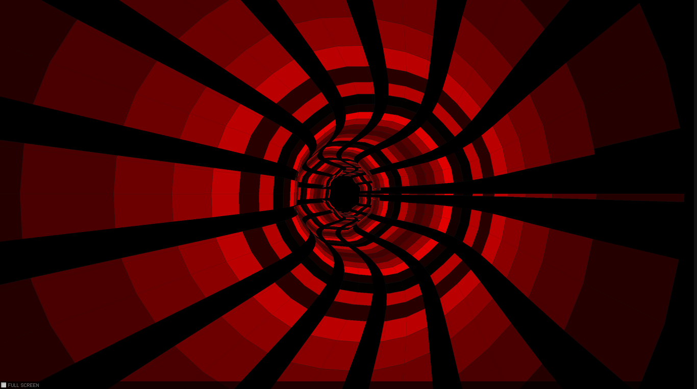
    And this is how it looks after implementation. By the way this is a good example of how robust and fast are <IGraphicsData> and drawGraphicsData functions combined.

    (Move the mouse to change the color shading intensity)

    After implementing the basic structure I thought – following the suggestion of some of the active members of wonderfl community – it would be nice to add some extra feature like sound visualization. Initially this little effect consists of some sinusoidally  curvy movement modifying the color intensity by the mouse position. You can check the effect by clicking on the image above.

    I was pleasantly surprised by the smoothly frame rate of the effect, so as i mentioned earlier the next step was to implement the algorithm for sound visualization. Thanks to makc3d audio API it was an easy job to obtain some samples which later could be used for the funky disco effect following the rhythm of the sound. This simple API connects to BeatPort portal, and by providing an unique key we can select from a various music genres. I opted for dubstep only because the high variation of beats can produce a very differentiated transition (a next step could be to implement an interface for selecting the different music channel).

    This is another variation.

    Playing with the values we can obtain different visualization effects. For example scaling up the bass bit rate we can obtain a nice upscaled flowing ring or reducing the radius value we should obtain a perfect circular cube like in the example below.

    Definitely a GUI interface would have been a better choice for playing with values, but because i put together this experiment in almost two hours i didn’t take the effort to polish the code. Maybe in a future time.

    (Scroll the mouse to jump to the next track)

    You can grab the source code here!

  • Cloth simulation with RK4 numerical integration

    Cloth simulation with RK4 numerical integration

    Click here to see it in action

    (click to see it in action)

    In this article I will discuss about something which is best known as numerical integration. I have always been fascinated by the cloth simulations, and wondered how it can be possible to reproduce this visually appealing effect using Actionscript, knowing that the AVM (Adobe Virtual Machine) is lacking well behind other languages like Java, not to mention C++ in terms of pure computation performance. Well to my surprise, after implementation I managed to obtain a pretty solid frame rate.

    The concept

    The core algorithm of the simulation is based on two concept known in physics as the Newton law’s of motion and restoration of force. This method is reasonably simple and robust and is a good general candidate for numerical solution of differential equations when combined with an intelligent adaptive step-size routine. After surfing the net for some tips and inspiration and reading Keith Peter’s book (AdvancED ActionScript 3.0 Animation), I got a grasp about the whole concept and physics acting behind it.

    The last temptation to implement my version came when I saw this amazing experiment implemented in Processing.

    The backbone of every clothing simulation is the so called numerical integration. There are many different techniques and implementation for physics simulation but, most of them use one of the three widespread integration method: Euler integration, Verlet integration and Runge-Kutta. The most significant difference between these methods consist in the accuracy of the movement.

    The Euler integration is the simplest one and uses the following algorithm: first calculate the actual position of the object, concatenate by the velocity and then apply acceleration. This is a very straightforward approximation with a very good performance, only it’s not accurate (unless we use an extremely small timestep size  – which we have no control over).

    The Verlet integration is very similar with Euler integration only this time we’ll get rid of the velocity component. We only need to calculate the change in position applying the acceleration value (A = F/m) which is a scalar component (the position and velocity actually are vectors). This is however velocity. So knowing the previous position and acceleration we could calculate the current position at the next frame. Keith Peters explain the differences between implementations in a very fashionable and enjoyable manner, so you should understand it easily. However my implementation differs quite enough from that one used in Keith’s book.

    Click to image

    (click to see it in action)

    The implementation

    In this experiment i’m gonna use Runge Kutta or simply RK4 implementation, but we can implement almost with the same accuracy the Verlet integration too. Very simply put, the algorithm first calculate the position and velocity at a certain interval (this calculation is done 4 times) and then make an approximation of them, and the average should be the object position and velocity at a certain position in time. The strength of this method is it’s accuracy, considering the minimal performance loss (i got almost constant 60 fps on my machine).

    Translated to AS3 it looks like this:

    /**
     * Get initial position, K1 velocity
     * apply forces and velocity, the result is K2
     */
    
    for (i = 0; i < numPart; i++)
    {
    	p = particles[i];
    
    	if (!p.fixed)
    	{
    		originalPos = originalPosV[i];
    		k1Vel = k1VelV[i];
    
    		s = (0.5 * t);
    		k1Vel.x *= s;
    		k1Vel.y *= s;
    		k1Vel.z *= s;
    		p.position.x = originalPos.x + k1Vel.x;
    		p.position.y = originalPos.y + k1Vel.y;
    		p.position.z = originalPos.z + k1Vel.z;
    
    		originalVel = originalVelV[i];
    		k1Force = k1ForceV[i];
    
    		s = (0.5 * t / p.mass);
    		k1Force.x *= s;
    		k1Force.y *= s;
    		k1Force.z *= s;
    		p.velocity.x = originalVel.x + k1Force.x;
    		p.velocity.y = originalVel.y + k1Force.y;
    		p.velocity.z = originalVel.z + k1Force.z;
    	}
    }
    
    particleSystem.applyForces();
    
    for (i = 0; i < numPart; i++)
    {
    	p = particles[i];
    
    	if (!p.fixed)
    	{
    		k2ForceV[i].x = p.force.x;
    		k2ForceV[i].y = p.force.y;
    		k2ForceV[i].z = p.force.z;
    		k2VelV[i].x = p.velocity.x;
    		k2VelV[i].y = p.velocity.y;
    		k2VelV[i].z = p.velocity.z;
    	}
    
    	p.force.x = 0;
    	p.force.y = 0;
    	p.force.z = 0;
    }
    
    /**
     * Get initial position, K2 velocity
     * apply forces and velocity, the result is K3
     */
    
    for (i = 0; i < numPart; i++)
    {
    	p = particles[i];
    
    	if (!p.fixed)
    	{
    		originalPos = originalPosV[i];
    		k2Vel = k2VelV[i];
    
    		s = (0.5 * t);
    		k2Vel.x *= s;
    		k2Vel.y *= s;
    		k2Vel.z *= s;
    		p.position.x = originalPos.x + k2Vel.x;
    		p.position.y = originalPos.y + k2Vel.y;
    		p.position.z = originalPos.z + k2Vel.z;
    
    		originalVel = originalVelV[i];
    		k2Force = k2ForceV[i];
    
    		s = (0.5 * t / p.mass);
    		k2Force.x *= s;
    		k2Force.y *= s;
    		k2Force.z *= s;
    		p.velocity.x = originalVel.x + k2Force.x;
    		p.velocity.y = originalVel.y + k2Force.y;
    		p.velocity.z = originalVel.z + k2Force.z;
    	}
    }
    
    particleSystem.applyForces();
    
    for (i = 0; i < numPart; i++)
    {
    	p = particles[i];
    
    	if (!p.fixed)
    	{
    		k3ForceV[i].x = p.force.x;
    		k3ForceV[i].y = p.force.y;
    		k3ForceV[i].z = p.force.z;
    		k3VelV[i].x = p.velocity.x;
    		k3VelV[i].y = p.velocity.y;
    		k3VelV[i].z = p.velocity.z;
    	}
    
    	p.force.x = 0;
    	p.force.y = 0;
    	p.force.z = 0;
    }
    
    /**
     * Get initial position, K3 velocity
     * apply forces and velocity, the result is K4
     */
    
    for (i = 0; i < numPart; i++)
    {
    	p = particles[i];
    
    	if (!p.fixed)
    	{
    		originalPos = originalPosV[i];
    		k3Vel = k3VelV[i];
    
    		s = (0.5 * t);
    		k3Vel.x *= s;
    		k3Vel.y *= s;
    		k3Vel.z *= s;
    		p.position.x = originalPos.x + k2Vel.x;
    		p.position.y = originalPos.y + k2Vel.y;
    		p.position.z = originalPos.z + k2Vel.z;
    
    		originalVel = originalVelV[i];
    		k3Force = k3ForceV[i];
    
    		s = (0.5 * t / p.mass);
    		k3Force.x *= s;
    		k3Force.y *= s;
    		k3Force.z *= s;
    		p.velocity.x = originalVel.x + k3Force.x;
    		p.velocity.y = originalVel.y + k3Force.y;
    		p.velocity.z = originalVel.z + k3Force.z;
    	}
    }
    
    particleSystem.applyForces();
    
    for (i = 0; i < numPart; i++)
    {
    	p = particles[i];
    
    	if (!p.fixed)
    	{
    		k4ForceV[i].x = p.force.x;
    		k4ForceV[i].y = p.force.y;
    		k4ForceV[i].z = p.force.z;
    		k4VelV[i].x = p.velocity.x;
    		k4VelV[i].y = p.velocity.y;
    		k4VelV[i].z = p.velocity.z;
    	}
    
    	p.force.x = 0;
    	p.force.y = 0;
    	p.force.z = 0;
    }
    
    /**
     * Update initial position and velocity based on intermediate values
     */
    
    for (i = 0; i < numPart; i++)
    {
    	p = particles[i];
    
    	if (!p.fixed)
    	{
    		//position
    
    		originalPos = originalPosV[i];
    		k1Vel = k1VelV[i];
    		k2Vel = k2VelV[i];
    		k3Vel = k3VelV[i];
    		k4Vel = k4VelV[i];
    
    		k2VelInt.x = k2Vel.x;
    		k2VelInt.y = k2Vel.y;
    		k2VelInt.z = k2Vel.z;
    		s = (2);
    		k2VelInt.x *= s;
    		k2VelInt.y *= s;
    		k2VelInt.z *= s;
    
    		k3VelInt.x = k3Vel.x;
    		k3VelInt.y = k3Vel.y;
    		k3VelInt.z = k3Vel.z;
    		s = (2);
    		k3VelInt.x *= s;
    		k3VelInt.y *= s;
    		k3VelInt.z *= s;
    
    		intVel.x = k1Vel.x + k2Vel.x + k3Vel.x + k4Vel.x;
    		intVel.y = k1Vel.y + k2Vel.y + k3Vel.y + k4Vel.y;
    		intVel.z = k1Vel.z + k2Vel.z + k3Vel.z + k4Vel.z;
    		s = (t / 6);
    		intVel.x *= s;
    		intVel.y *= s;
    		intVel.z *= s;
    		p.position.x = originalPos.x + intVel.x;
    		p.position.y = originalPos.y + intVel.y;
    		p.position.z = originalPos.z + intVel.z;
    
    		// velocity
    
    		originalVel = originalVelV[i];
    		k1Force = k1ForceV[i];
    		k2Force = k2ForceV[i];
    		k3Force = k3ForceV[i];
    		k4Force = k4ForceV[i];
    
    		k2ForceInt.x = k2Force.x;
    		k2ForceInt.y = k2Force.y;
    		k2ForceInt.z = k2Force.z;
    		s = (2);
    		k2ForceInt.x *= s;
    		k2ForceInt.y *= s;
    		k2ForceInt.z *= s;
    
    		k3ForceInt.x = k3Force.x;
    		k3ForceInt.y = k3Force.y;
    		k3ForceInt.z = k3Force.z;
    		s = (2);
    		k3ForceInt.x *= s;
    		k3ForceInt.y *= s;
    		k3ForceInt.z *= s;
    
    		intForce.x = k1Force.x + k2Force.x + k3Force.x + k4Force.x;
    		intForce.y = k1Force.y + k2Force.y + k3Force.y + k4Force.y;
    		intForce.z = k1Force.z + k2Force.z + k3Force.z + k4Force.z;
    		s = (t / 6 * p.mass);
    		intForce.x *= s;
    		intForce.y *= s;
    		intForce.z *= s;
    		p.velocity.x = originalVel.x + intForce.x;
    		p.velocity.y = originalVel.y + intForce.y;
    		p.velocity.z = originalVel.z + intForce.z;
    	}
    }

    (For a comparison between different numerical integration methods read this article: http://codeflow.org/entries/2010/aug/28/integration-by-example-euler-vs-verlet-vs-runge-kutta/.)

    Here is the final result (press space to show/hide the stats).

    Press right arrow to show wire frame and texture simultaneously, up arrow to show only bitmap texture and left arrow to show only the wire-frame.