Category: Tutorials

  • Porting Pigo face detection library to Webassembly (WASM)

    Porting Pigo face detection library to Webassembly (WASM)

    Pigo Wasm

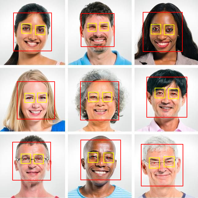
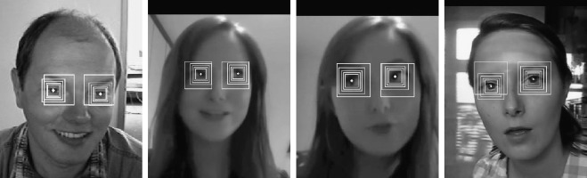
    In the last couple of occasions I wrote about the Pigo face detection library I have developed in Go. This article is another one from the series, but this time I’m focusing on WASM (Webassambly) integration. This is another key milestone in the library evolution, considering that when I started this project the library was capable only for face detection. Later on the library has been extended to support pupils/eyes localization, then facial landmark points detection and it has also been adapted to be integrated into different programming languages as a shared object library (SO). I’m pretty delighted about the great acceptance and support received during the development from the programming community, the library being featured a couple of times in https://golangweekly.com/, received 2.5k stars on the repo Github page (and still counting), getting many positive feedback on Reddit, which means it payed back the efforts.

    But first what is WASM? To quote the https://webassembly.org/ homepage:

    Quote leftWebAssembly (abbreviated Wasm) is a binary instruction format for a stack-based virtual machine. Wasm is designed as a portable target for compilation of high-level languages like C/C++/Rust, enabling deployment on the web for client and server applications.Quote right

    In other words this means that compiling and porting a native application to the WASM standard will give the generated web application a speed almost equal to the native one.

    Starting from v1.11 an experimental support for WASM has been included into the Go language, which has been extended on v1.12 and v1.13. As I mentioned in the previous articles Go suffers terrible in terms of native and platform agnostic webcam support and as of my knowledge currently there is no single webcam library in the Go ecosystem which is platform independent. This was the reason why, to prove the library real time face detection capabilities, I opted to lean on exporting the main function as a shared object library, but lately this proved to be inefficient in terms of real time performance, since on each frame the Python app had to transfer the pixel array to the Go app (where the face detection operation is happening) and get back the detected faces coordinates. Of course because of the two way (back and forth) communication, this process fall back considerably in terms of pure performance.

    WASM to the rescue

    As I mentioned above starting from v1.11 the standard Go code base now includes the syscall/js package which targets WASM. However the API has been refactored and gone trough a few iterations to became stable as of v1.13. This also means that the WASM API of v1.13 is no more compatible with the v1.11. The API became so mature that there is no need to use external libraries targeting the Javascript runtime in Go, like Gopherjs.

    In order to compile for Webassambly we need to explicitly specify and set the GOOS=js and GOARCH=wasm environment variables on the building process. Running the below command will build the package and produce a .wasm executable Webassambly module file.

    $ GOOS=js GOARCH=wasm go build -o lib.wasm wasm.go

    This file then can be referenced in the main html file.

    That’s the only thing we need to do in order to have fully functional WASM application. The hardest part is coming afterwards. When we are targeting WASM there are a few takeaways we need to keep in mind in order the implementation to run as smooth as possible:

    1. To have access to a Javascript global variable in Go we have to call the js.Global() function.
    2. To call a JS object method we have to use the Call() function.
    3. To get or set an attribute of a JS object or Html element we can call the Get() or Set() functions.
    4. Probably the trickiest part of the Go Wasm port is related to the callback functions, and there are a lot of places where we need to take care of them. One of the most important one is the canvas requestAnimationFrame method, which accepts as a second argument a callback function. Now to invoke this method in Go we need to apply to the js.FuncOf(func(this js.Value, args []js.Value) interface{}{...} function, where the second argument is the callback function argument. A very important note: the function body should be called inside a goroutine, otherwise you’ll get a deadlock runtime exception. You can check the package documentation here: https://godoc.org/syscall/js

    The implementation details

    Now let’s take a deep breath and roll into the implementation details. One of the key components of the face detection application is the binary cascade file parser. Since in normal circumstances, when we are fetching and parsing the binary files locally, we can rely on the os system package, this is not the case on WASM, because we do not have access to the system environment. This means that we cannot load and parse the files sitting on our local storage. We need to fetch them through the supported Javascript methods like the fetch method. In Javascript this method returns a promise with two arguments: a success and a failure. As I mentioned previously the callback functions needs to be invoked in separate goroutines and the most straightforward way to orchestrate the results when we are dealing with goroutines is to use channels. So the fetch method should return the parsed binary file as a byte array and an error in case of a failure.

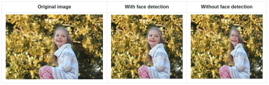
    The rest of the implementation does not differ in anything from the Unpack() method presented in the previous article. Once we get binary array there is nothing left over just to unpack the cascade file, transform it to the desired shape and extract the relevant information.

    I won’t go into too much details about the detection algorithm itself, since I’ve discussed it in the previous articles. I will detail what’s most important in the perspective of the WASM integration. Another key importance part in the WASM integration is related to the webcam rendering operation. In Javascript we can access the webcam in the following way:

    We can translate this snippet to Go (WASM) code in the following way:

    This will return a canvas object (struct) over it we can call the rendering method itself. In the background this will trigger the requestAnimationFrame JS method, drawing each webcam frame to a dynamically created image element. From there we can extract the pixel values calling the getImageData HTML5 canvas method. Since this will return an object of type ImageData which values are of Uint8ClampedArray, these needs to be converted to a type supported by the Go WASM API. The only supported uint type in the Go syscall/js API is uint8, so the most suitable way is to convert the Uint8ClampedArray to Uint8Array. We can do this by calling the following method:

    The code below shows the rendering method. It’s a pretty common Javascript code adapted to WASM Go, including the code responsible for the face detection, but this have been discussed in the previous articles. The most important part is the type conversion, without that we are just getting a compiler error.

    And to put all together, in the main function we are just calling the webcam Render() method, once the webcam has been initialized, otherwise an alert telling that the webcam was not detected.


    The end result

    Voila, we are done. Here is how the Webassambly version of Pigo looks like in realtime. Pretty good, huh? That’s, all, thanks for reading and if you like my works you can follow me on Twitter or give it a star on the project Github repo: https://github.com/esimov/pigo.

  • Pupils/eyes localization in the Pigo face detection library

    Pupils/eyes localization in the Pigo face detection library

    In the previous post I’ve presented a general overview of the Pigo face detection library I’m working on, some examples of how you can run it on various platforms and environment for detecting faces and also its desired scope in the Go ecosystem. Meantime the library got a huge revamp and reached a new milestone in the development live cycle, which means as of today Pigo is capable of pupils/eyes localization and even better supports facial landmark points detection. In this article I will focus on the pupils/eyes detection, following that in the next article aiming to discuss about the facial landmark points detection. So let’s get started.

    Pupils/eyes localization

    The implementation is based on the Eye pupil localization with an ensemble of randomized trees paper, which pretty much resembles with the method used on face detection but with few remarkable differences. I will explain them shortly. Both of the implementations are based on tree ensembles, well known for achieving impressive results, in contrary to a single tree detection method. This means that the classifier used for the pupil/eyes detection is generated based on decision trees and the training data is recursively clustered in this fashion until some termination condition is met.

    Since we know the leaf structure of the binary classifier the only thing we need to do is to decompose it in order to obtain the data structure. The decomposition procedure is based on the following steps:

    • Read the depth (size) of each tree and write it into the buffer array.
    • Get the number of stages as 32-bit unsigned integers and write it into the buffer array.
    • Obtain the scale multiplier (applied after each stage) and write it into the buffer array.
    • Obtain the number of trees per stage and write it into the buffer array.
    • Obtain the depth of each tree and write it into the buffer array.
    • Traverse all the stages of the binary tree, traverse all the branches of each stage and read prediction from tree’s leaf nodes.

    The returned element should be a struct containing all of the above information.

    There is a problem though: the output of the regression trees might be noisy and unreliable in some special cases like when we are feeding some low quality video frames or images. This is the reason why the method introduces a random perturbation factor during runtime to outweigh the false positive rates on detection. Later on, after the detected face region is classified we sort the perturbations in ascendant order and retrieve the median value of the resulted vector.

    Pupil localization with perturbation

    The classification procedure consists in the following: traverse the trees on all the stages and use almost the same binary test applied on the face classification procedure. We have to restrict the pupils/eyes classification method exclusive to the detected face region. In the end we will obtain the pupils coordinates and a scale factor. The scale factor is less important in this case, since it’s useful only if we wish to give a different size for the detected pupils.

    We are using the same method for left and right eye detection, the only difference is that for the right eye detection we flip the sign in the following formula.

    To run it on static images a CLI application is bundled into the library. The difference from the face detection is that in addition we have to provide the binary classifier for pupil/eyes detection. Since the library is constructed in a modular fashion, this means that only certain sections needs to be extended like the binary parser and the classification function. Other parts of the code remains pretty much unchanged.

    This is how the end result looks like:

    Pupils/eyes detection

    Webcam demo

    I have also created a webcam demo running in Python, since as of today there isn’t a native Go webcam library supported on all platforms. The major takeaway is that the computational (the face and pupils detection) part is executed in Go and the resulted data (the detection coordinates) are transferred to Python through a shared object library.

    It sounds like an alchemy, but it’s definitely a working solution. On the Go part there are a few things we need to take care.

    • The exported function should be annotated with the //export statement.
    • The source must import the pseudo C package.
    • An empty main function should be declared.
    • The package must be a main package.

    These are only the technical requirements imposed by the language in order to transfer the Go code as a shared object. Afterwards we can build the program with the following commands (in fact these will be executed from the Python code).

    To communicate with the Go code from the Python code base we will use the Ctype library. This is a handy library which provides C compatible data types, and allows calling functions in DLLs or shared libraries. Using the library at first might be intimidating since it heavily relies on the C structs and types. Also accessing the Go data is possible exclusively through pointer interfaces. This means we need to be aware about the data type, the buffer length and the maximum capacity of the transferred Go slice. In fact the slice will be a pointer pointing to a data structure. In Python we have to declare a class which maps to a C type struct having the following components:

    On the other hand at the Go counterpart after running the detection function and retrieving the coordinate results we need to convert them as one dimensional array, since in Go is not possible transfer a 2D array over an array pointer. The trick is to convert the 2D array (since we are dealing with multiple face detection and by default multiple pupils/eyes detection) to a 1D array in such a way to delimit the detection groups from each other. One efficient way to make this happen is to introduce as a first slice element the number of detected faces. Since we know how many faces are detected, later on in the Python part we can transform the array with the help of numpy to the desired shape.

    This is how the Go code looks like. We are invoking the runtime.KeepAlive(coords) function to make sure the coords is not freed up by the garbage collector prematurely.

    In the end we should obtain something like below, where the first value represent the number of the detected faces and the rest of the values are the x and y coordinates and the scale factor of the detected faces, respectively pupils.

    [2 0 0 0 0 272 297 213 41 1 248 258 27 41 0 248 341 27 41 0 238 599 72 25 1 230 587 9 25 0 233 616 9 25 0]

    Back to Python. We are capturing each frame from the webcam and transferring the underlying binary data to Go as a byte array. After running the face detector over the obtained binary data we are retrieving back the obtained one dimensional array. Ctypes requires to define a class which must contains a _field_ attribute. This attribute must be a list of 2-tuples, containing a field name and a field type. Since the Go slice has a len and a cap attribute we will define them as the tuple elements. Once we’ve defined the base class we also have to define the argument types. The argument type will be the base class and the return type will be a pointer type, represented as integer exactly as the Go return type.

    Since in Ctypes we are dealing with pointer values, this means we do not have any information about the allocated buffer size needed by the face detector, this is the reason why we are allocating a buffer just enough to hold all the values returned by the detector. Later on we’ll trim the buffer length by emptying the null values. We can do this because we already know the number of detected faces. So the end results will be the number of detected faces multiplied by 3, since each face detection result should be extended with a pair of pupil detection.

    And that’s all. Below is a video capture of running the face detector in real time. The small lagging is due to time needed to convert the Go code to a shared library, otherwise the algorithm can produce much higher frame rates.

    I hope that you enjoyed reading this article and got a better understanding of the interaction between Go and Python. In the next article I’ll present a concrete example using this feature. If you appreciate the work done on this library please show your support by staring the library Github repository here: https://github.com/esimov/pigo.

  • Technical overview of Pigo face detection library

    Technical overview of Pigo face detection library

    Pigo Logo

    Pigo’s cute logo

    Pigo is a pure face detection library implemented in and for Go and it is based on Pixel Intensity Comparison-based Object detection paper (https://arxiv.org/pdf/1305.4537.pdf). Pigo has been around for more than a year, but I haven’t published a technical article about the library, so I thought it was time to fill in the gap.

    Technical overview

    The first and foremost question: what was the motivation and the purpose of making this library, since GoCV does exists from a quite a long time in the Go ecosystem and is trying to be the perfect toolset for everyone who is willing to combine the simplicity of the Go language with the comprehensiveness of OpenCV in everything related to computer vision, machine learning and anything between?

    Making a quick search on the web for face detection with Go, almost 100% of the returned results are C bindings to external libraries. Pigo is making an exception from this, since it is purely developed in Go, having in mind the casual Go developer. The reference implementation is written in C and is available here: https://github.com/nenadmarkus/pico. There is no need to install platform dependent libraries, no need to compile and build the giant, monolithic OpenCV package.

    What are the benefits of using Pigo? Just to name a few of them:

    • High processing speed
    • No need for image preprocessing prior detection
    • No need for the computation of integral images, image pyramid, HOG pyramid or any other similar data structure
    • The face detection is based on pixel intensity comparison encoded in the binary file tree structure
    • Fast detection of in-plane rotated faces

    New let’s see what are the similarities and what are the differences between Pigo and other detection methods. Similar to the Viola Jones face detection algorithm, Pigo is still using cascade decision trees at all reasonable scales and positions, but the cascade classifier is in binary format. The role of a classifier is to tell if a face is present in current region or not. The classifier consists of a decision tree where the leaves or internal nodes contains the results of pixel intensity comparison test in binary format. The binary test can be expressed with the following formula:

    \( bintest(R, \text{$x1$, $y1$, $x2$, $y2$}) =
    \begin{cases}
    0, & \text{$R$[$x1$, $y1$]} \le \text{$R$[$x2$, $y2$]} \\
    1, & \text{otherwise},
    \end{cases}
    \)

    where \(R\) is an image region and (\(x_i\), \(y_i\)) represents the normalized pixel location coordinates, which means that the binary test can be easily resized if needed.

    Since the cascades are encoded into a binary tree, this means that in order to run the detection method the cascade classifier needs to be unpacked. In the end the unpacking method will return a struct which has the following elements:

    Due to many regions present in the image, the decision trees are organized in cascading classifiers, making each member of cascade to be evaluated in \( O(1) \) time with respect to the size of the region. An image region is considered being face if it passes all the cascade members. Since this process is limited to a relatively small number of regions, this gains high computation speed.

    The above method will classify the cascade trees based on the trained data, but since many of them are in-plane faces, this means that rotated faces are not detectable. For this reason we need to introduce another method, which classifies the regions based on the rotation angle provided as input. (I’m not including the code snippet for this one, since you can check it on the source code.)

    Another key aspect of the algorithm is that during the decision tree scanning, each detection is flagged with a detection score. An image region is considered being face if the detection score average is above a certain threshold (in general around 0.995). All regions below this threshold are not considered to be faces. We can achieve different ratios of true positives to false positives by varying the threshold value. Since the detector is based on pixel intensity comparison, this means that it’s also sensible to small perturbations and variations of the underlying pixel data, influenced mostly by the scaling and the rotation of the objects, resulting overlaps in detections.

    Face detection without clustering

    The detection results without the clustering applied

    This is the reason why the cascade detections are clustered together in a post processing step and the final result is produced by applying the intersection over union formula on the detected clusters.

    In return this does not provide the rectangle coordinates of the detected faces as expected, but a slice of Detection struct consisting of number of rows and columns, the scale factor and the detection score. To translate from these to the standard image.Rectangle is only a matter of a simple conversion realized as in the following lines:

    And this is how the final output looks like after the detection results have been clustered.

    The detection results with the clustering applied

    Pigo and GoCV comparison

    The best way to compare the two libraries is to measure them both in terms of pure performance, detection speed but also accuracy. The most obvious way to evaluate them is to run some benchmarks with the same prerequisites. One thing to note is that the classifier is set to detect faces on the same image over and over again. This is to get an accurate idea of how well the algorithm performs.

    To have a more accurate benchmark and to measure only the execution time the b.ResetTimer() is called to reset the timer so the setup is not counted towards the benchmark.

    Here are the results:

    For the above test we were using a sample image with a Nasa crew of 17 persons. Both of the libraries have returned exactly the same results, but Pigo was faster and also the memory allocation was way less compared to GoCV.

    Use cases

    To demonstrate the real time capabilities of the Pigo face detection library and also to show how easily could be integrated into let’s say a Python project I have created a couple of use cases, targeting different kinds of applications. The first one is the usual face detection example: real time, webcam based face detection, marking the detected faces with a rectangle (or circle).

    Using Pigo as a shared object library

    Go running in Python? Yes, that’s true: we are harvesting the Go feature to export binary files as shared objects. The Go compiler is capable of creating C-style dynamic shared libraries using build flag -buildmode=c-shared. Running the go program with the following flag will generate the shared object library which later on can be imported into the Python program. But the following conditions must be satisfied:

    • The exported function should be annotated with the //export statement.
    • The source must import the pseudo C package.
    • An empty main function should be declared.
    • The package must be a main package.

    Knowing the above conditions we can execute a shell command from the Python program which in the end will call the shared object library returning the detection results. Later on we can operate with the values obtained. Below is an example of the process just described, whose source code and other examples can be found on the project examples directory: https://github.com/esimov/pigo/tree/master/examples.

    Another handy application I have created is to blur out the detected faces. For static images we can lean on stackblur-go library to blur out the detected faces, otherwise if we are using as a shared library, which is getting imported into a Python program, then we can make use of OpenCV blur method.

    I have also successfully integrated Pigo into Caire, the content aware image resizing library I have created. Thanks to Pigo it was possible to avoid the face distortions by restricting the seam removing algorithm only to the picture zones without faces. Once we’ve detected the faces it was only a piece of cake to exclude them from the processing. For more information about Caire read my other blog post, where I’ve detailed in large how the seam carving algorithm is working.

    Serverless integration

    Pigo has been successfully integrated into the OpenFaaS platform, easing you out from all the tedious work requested by the installation, configuration of the Go language etc., making possible to expose it as an FaaS function. This means once you have an OpenFaaS platform installed on your local machine with only two commands you have a fully working docker image where Pigo can be used as a serverless function.

    OpenFaaS user interface

    The OpenFaaS user interface

    Pigo OpenFaaS result

    The faceblur function applied over an input image

    Below are some of the OpenFaaS functions i have created integrating Pigo:

    https://github.com/esimov/pigo-openfaas-faceblur

    https://github.com/esimov/pigo-openfaas

    The docker image is also available on the docker hub, having already more then 10k+ downloads. https://cloud.docker.com/u/esimov/repository/docker/esimov/pigo-openfaas

    Summary

    In conclusion as you might realize Pigo is a lightweight, but full fledged face detection library, easy to use and easy to integrate into different platforms and environments, having a simple API, but well enough for making the job done.

    For more computer vision, image processing and creative programming stuffs you can follow me on twitter: https://twitter.com/simo_endre

  • Coherent Line Drawing implementation in Go (GoCV)

    Coherent Line Drawing implementation in Go (GoCV)

    Surfing the web a beautiful, pencil-drawn like image captured my attention, it looked like as a hand-drawn image, but also became almost evident that it was a computer generated art. I found that it was created using an algorithm known as Coherent Line Drawing.

    Coherent Line Drawing

    Introduction

    In the last period of time I have been working on and off (as my limited free time permitted) on the implementation of the Coherent Line Drawing algorithm developed by Kang et al. Only now I considered that the implementation is so stable that I can publish it, so here it is: https://github.com/esimov/colidr.

    Since my language of choice was Go I decided to give it a try implementing the original paper in Go, more explicitly in GoCV, an OpenCV wrapper for Go. I opted for this choice since the implementation is heavily based on linear algebra concepts and requires to work with matrices and vector spaces, things in what OpenCV notoriously excels.

    However some of the functions required by the algorithm were missing from the GoCV codebase (at that period of time) like Sobel, uniformly-distributed random numbers and also vector operations like getting and setting the vector values. Meantime checking the latest release I found that the core codebase has been extended with some of the missing functionalities like the Sobel threshold, bitwise operations etc., however there were still missing pieces required by the algorithm. For this reason I have extended the GoCV code base with the missing OpenCV functionalities and included into the project as vendor dependency. Probably in the upcoming future I will create a pull request to merge it back in the main repository.

    I won’t go into too much detail about the algorithm itself, you can find it in the original paper. I will discuss mostly about the technical difficulties encountered during the implementation, but also about the challenges imposed by gocv and OpenCV.

    Why Go?

    Now let’s talk about the challenges imposed by the project. The first question which might arise is why in Go, knowing that Go is not really appealing for creative coding, and it is mostly used in automatization, infrastructure, devops and web programming.

    From my first acquaintance with Go (which was quite a few years back) I was intrigued by the potential possibilities offered by the language to make use of it in fields like image processing, computer vision, creative coding etc, since these are the fields i’m mostly interested in, and almost all of my open source project developed in Go have circulated around this topic. So this project was another attempt of mine to demonstrate that the language is well suited for these kind of projects too.

    Go has a small package for image operations, but it is fair enough for anything you need to read an image file, obtain and manipulate the pixel values and finally to encode the result into an output file. Everything is concise and well structured. Since in this project we mostly rely on the OpenCV embedded functions provided by GoCV, there are still plenty of use cases when you need to rely on the core image library. Go does not provide a high level, abstract function to modify the source image, you need to access the raw pixel values in order to modify them.

    Another key aspect in the language choice was that Go has an out of the box command line flag parsing library, just what I needed, since I conceived this application to be executed from the terminal. Maybe in the upcoming future I will create a GUI version too.

    Technical challenges

    Going back to the technical challenges I encountered during the implementation, one of the main headaches was related to how sensible OpenCV is to the way the types of matrices are declared. I was banging my head into the wall many times for the simple reason that my matrices were defined as gocv.MatTypeCV32F, however they should have been defined as gocv.MatTypeCV32F+gocv.MatChannels3, since the concatenation of these two variables were producing the desired matrix type value declared in the underlying OpenCV code base. More exactly by creating a new Mat and defining it’s type as simply MatTypeCV32F, the underlying gocv method will call the Mat_NewWithSize C method, having the last parameter the type of the matrix. Exactly this kind of limitation have confused me, ie. not all of the supported OpenCV mat types have been defined in the GoCV counterpart.

    Since OpenCV is very flexible on matrix operations and won’t complain about the matrix conversions from one type to another, there are some edge cases when they are producing undesired results. This is a thing you have to consider when you are doing matrix operations in OpenCV: you need to be aware of the matrix type, otherwise your end results could be utterly compromised.

    However comparing the OpenCV and GoCV matrix type tables, a lot of types are still missing from GoCV. For this simple “thing” my outputs were far from desirable from what it should have been. I was spinning in round and round, going back and forth, trying different solutions, comparing the code with the pseudo algorithms and formulas provided in the original paper to finally realizing that my matrices were defined with the wrong type or because some of the types declared in OpenCV were completely missing from the GoCV counterpart. The solution was either to extend the core code base or to concatenate the two matrix types (as presented above) in order to produce the correct type value requested by OpenCV.

    Another elementary thing which is missing from GoCV is the SetVecAt method for setting or updating the vector values, even though a method for retrieving the vector values does exists. My initial attempt was to modify the vector values on byte level and encode it back into a matrix using the GoCV NewMatFromBytes method, which proved to be completely inefficient.

    The solution was to extend the core GoCV codebase with a SetVec method.

    Another thing I learned is converting one matrix type to another does not always work as you think. I experienced this issue when during the debugging session I had to convert a float64 matrix to uint8, which can be exported as a byte array needed for the final binary encoding. It worked, but converting back to a float64 matrix requested by rotateFlow method didn’t not produced the desired output. (This method applies a rotation angle on the original gradient field and calculates the new angles.)

    Since Go is using strict types for variable declarations, the auto casting is not possible like in C or C++. For this reason you need to pay attention to how you are converting the values from one type to another. Because GoCV / OpenCV matrices defined as floats are using 32 bits precision float values we need to be cautious when we have to cast a value defined as float64 for example to a 32 bit integer. This was the case on edge tangent flow visualization.

    The examples below were produced with the wrong (left) and good type casting (right).

    Flowfield wrong
    Flowfield good

    Even though the paper provided the implementation details for ETF visualization, my first attempt of it’s implementation didn’t produced the correct results. Only when I printed out the results I realized that the values were spanning over the range of the 32 bit integers, however OpenCV does not complained about this. The solution for this problem was to cast the index values of the for loop iterator as float32.

    This is a takeaway you have to consider when you are working with OpenCV matrix types, especially in a language like Go, which is very strict in terms of variable types definition.

    Conclusion

    To sum up: GoCV is a welcome addition for the Go ecosystem, considering that it is under development many of the core OpenCV features are already implemented. However as I mentioned above there are still missing features, which should be addressed to become a viable OpenCV wrapper for the Go ecosystem. What I have learned using OpenCV is that you have to tinker with the values, and slight changes on the inputs can produce completely broken outputs, so you need to find that tiny middle road where the different equation parameters can converge.

    Sample images

    Great Wave
    Great Wave
    Starry Night
    Starry Night
    Happy people
    Happy people
    Tiger
    Tiger

    Source code

    The code is open source and can be found on my Github page:

    https://github.com/esimov/colidr

    You can follow me on twitter too: https://twitter.com/simo_endre

  • Caire – a content aware image resize library

    Caire – a content aware image resize library

    Let’s assume you want to resize an image without content distortion but also you wish to preserve the relevant image parts. The normal image resize, but also the content cropping technique is not really suitable for this kind of task, since the first one will simply resize the image by preserving the aspect ratio and the last one will crop the image on the defined coordinate section, which might results in content loss, especially on photos with the relevant information scattered trough the image. Not even the smart cropping technique will help too much in this case.

    This is what Caire, my content aware image resizing library developed in Go is trying to remedy. I’is pretty much based on the article Seam Carving for Content-Aware Image Resizing by Shai Avidan and Ariel Shamir.

    The background

    Let’s consider the image below (Fig.1). It’s a nice and clean picture with a wide open background. Now suppose that we want to make it smaller. We have two options: either to crop it, or to scale it. Cropping is limited since it can only remove pixels from the image periphery. Also advanced cropping features like smart cropping cannot resolve our issue, since it will remove the person from the left margin or will crop a small part from the castle. Certainly we do not want this to happen. Scaling also is not sufficient since it is not aware of the image content and typically can be applied only uniformly.

    Fig.1: Sample image

    Seam carving was developed typically for this kind of use cases. It works by establishing a number of seams (a connected path of low energy pixels) crossing the image from top to down or from left to right defining the importance of pixels. By successively removing or inserting seams we can reduce or enlarge the size of the image in both directions. Fig.2. Illustrates the process.

    Fig.2: The seam carving method illustrated

    First let’s skim through the details and summarize the important steps.

    • An energy map (edge detection) is generated from the provided image.
    • The algorithm tries to find the least important parts of the image taking into account the lowest energy values.
    • Using a dynamic programming approach the algorithm will generate individual seams crossing the image from top to down, or from left to right (depending on the horizontal or vertical resizing) and will allocate for each seam a custom value, the least important pixels having the lowest energy cost and the most important ones having the highest cost.
    • Traverse the image from the second row to the last row and compute the cumulative minimum energy for all possible connected seams for each entry.
    • The minimum energy level is calculated by summing up the current pixel value with the lowest value of the neighboring pixels from the previous row.
    • Traverse the image from top to bottom (or from left to right in case of vertical resizing) and compute the minimum energy level. For each pixel in a row we compute the energy of the current pixel plus the energy of one of the three possible pixels above it.
    • Find the lowest cost seam from the energy matrix starting from the last row and remove it.
    • Repeat the process.

    Implementation

    Seam carving can support several types of energy functions such as gradient magnitude, entropy, sobel filter, each of them having something in common: it values a pixel by measuring its contrast with its neighboring pixels. We will use the Sobel filter operator in our case. Typically in image processing the Sobel operator is used to detect image edges. It’s working with an energy distribution matrix to differentiate the sensitive image information from the less sensitive ones. (Fig. 3)

    Fig.3: Sobel threshold applied to the original image

    Once we obtained the energy distribution matrix we can advance to the next step to generate individual seams of one pixel wide. We’ll use a dynamic programming approach to store the results of sub-calculations in order to simplify calculating the more complex ones. For this purpose we define some setter and getter methods whose role are to set and get the pixel energy value.

    After generating the energy map there are two important steps we need to follow:

    Traverse the image from the second row to the last one and compute the cumulative minimum energy M for all possible connected seams for each entry (i, j). M is the two dimensional array of cumulative energies we are building up. The minimum energy level is calculated by summing up the current pixel value with the minimum pixel value of the neighboring pixels obtained from the previous row. This can be done via Dijkstra’s algorithm. Suppose that we have a matrix with the following values:

    Original matrix

    To compute the minimum cumulative energies of the second row we start with the columns from the first row and sum up with the minimum value of the neighboring cells from the second row. After the above operation is carried out for every pixel in the second row, we go to the third row and so on.

    Using Dijkstra’s algorithm to calculate the minimum energy values.

    Once we calculated the minimum energy values for each row, we select the last row as starting position and search for the pixel with the smallest cumulative energy value. Then we traverse up on the matrix table one row at once and again search for the minimum cumulative energy value up until the first row. The obtained values (pixels) make up the seam which should be removed.

    To remove the seam is only a matter of obtaining the pixel coordinates of the seam values and checking on each iteration if the processed pixel coordinates corresponds with the seams pixel values position. We can check the accuracy of our logic by drawing the removable seams on top of the image. (Fig.4)

    Fig.4: Low energy seams crossing the image

    The same logic can be applied to enlarge images, only this time we compute the optimal vertical or horizontal seam (s) and duplicate the pixels of s by averaging them with their left and right neighbors (top and bottom in the horizontal case).

    Fig.5: The final resized image

    Prevent face deformation with face detection

    For certain content such as faces when relations between features are important, automatic face detection can be used to identify the areas that needs protection. This is an important requirement since in certain situations when sensible image regions like faces (detected by the sobel filter operator) are compressed in a small area it might happen to get distorted (see Fig.6). To prevent this, once these regions are detected we can increase the pixel intensity to a very high level before running the edge detector. This way we can assure that the sobel detector will consider these regions as important ones, which also means that they will receive high energy values.

    Fig.6: Resizing image with and without face detection

    Below you can see the seam carving algorithm in action, first checking for human faces prior resizing the image. It’s visible from the image that the seams are trying to avoid the face zone normally marked with a rectangle. And this is done with a simple trick: if face zone is detected that rectangle is marked with a white background which makes the detector to believe that it’s an area with high energy map. For face detection it was used Pigo, another Go library developed by me.

    Conclusion

    Seam carving is a technique which can be used on a variety of image manipulations including aspect ratio change, image retargeting, object removal or even content amplification. Also it can be seamlessly integrated with a Convolutional Neural Network which can be trained for specific object recognition, making the perfect toolset for every content delivery solution. There are other numerous possible domains this technique could be applied or even extended like video resizing or the ability for continuous resizing in real time.

    Of course as every technology has its limitations, like the case when the processed image is very condensed, in the sense that it does not contain “less” important areas, ugly artifacts might appear. Also the algorithm does not perform very well when the image albeit being not very condensed, the content is laid out in a manner that it does not permit the seams from bypassing some important parts. In certain situations by tweaking the parameters, like using a higher sobel threshold or applying a blur filter these kind of limitations could be surpassed.

    Source code

    The code is open sourced and can be found on my Github page:

    https://github.com/esimov/caire

    https://github.com/esimov/pigo

  • Delaunay image triangulation

    Delaunay image triangulation

    In this article we present a technique to triangulate source images, converting them to abstract, someway artistic images composed of tiles of triangles. This will be an attempt to explore the fields between computer technology and art.

    But first, what is triangulation? Simply spoken a triangulation partitions a polygon into triangles which allows, for instance, to compute the area of a polygon and execute some operations on the computed polygon surface. In other terms the triangulation might be conceived as a geometric object defined by a point set, but what differentiates the polygons from a point set is the latter does not have an interior, except if we treat the point set as a convex hull/polygon. But to think of a point set as a convex polygon, the points from the interior of the convex hull should not be ignored completely. This is what differentiates the Delaunay triangulation from the other triangulation techniques.

    Fig.1: Point set triangulation.

    Delaunay triangulation

    Wikipedia has a very succinct definition of the Delaunay triangulation:

    … a Delaunay triangulation (also known as a Delone triangulation) for a given set P of discrete points in a plane is a triangulation DT(P) such that no point in P is inside the circumcircle of any triangle in DT(P)

    The circumcircle of a triangle is the unique circle passing through all the vertices of the triangle. This will get valuable meaning in the following. So considering that we have a set of six points we can obtain a triangulated polygon by tracing a circle around each vertex of the constructed triangle in such a manner that the circumcircle of all five triangles are empty. We also say, that the triangles satisfy the empty circle property (Fig.2).

    Fig.2: All triangles satisfy the empty circle property.

    After a short theoretical introduction now we want to apply this technique to a more practical but at the same time aesthetical field, concretely to transform a source image to it’s triangulated counterpart. Having the basic idea and it’s theoretical background we can start to construct the basic building blocks of the algorithm.

    Above all a short notice: we use Go as programming language for the implementation. First, because it has a very clean and easy to use API, second because it can be well suited for a CLI based application, which single scope is to convert an input file to a destination object.

    The algorithm

    Now into the algorithm. As the basic components are triangles we define a Triangle structs, having as constituents the nodes, it’s edges and the circumcircle which describes the triangle circumference.

    
    type Triangle struct {
          Nodes  []Node
          edges  []edge
          circle circle
    }
    

    Next we create the circumscribed circle of this triangle. The circumcircle of a triangle is the circle which has the three vertices of the triangle lying on its circumference. Once we have the circle center point we can calculate the distance between the node points and the triangle circumcircle. Then we can calculate the circle radius.

    We can transpose this into the following Go code:

    The question is how do we get the triangle points from the input image? To obtain a large triangle distribution on the image parts with more details we need somehow to analyze the image and mark the sensitive information. How do we do that? Sobel filter operator on the rescue. The Sobel operator is used in image processing to detect image edges. It’s working with an energy distribution matrix to differentiate the sensitive image informations from the less sensitive ones.

    Fig.3: Sobel operator applied to the source image.

    Once we obtained the sobel image we can sparse the triangle points randomly by applying some threshold value. At the end we obtain an array of randomly distributed points, but these points are more dense on the sensitive image parts, and scarce on less sensitive ones.

    Having the edge points we check whether the points are inside the triangle circumcircle or not. We save the triangle edges in case they are included and carry over otherwise. Then in a loop we search for (almost) identical edges and remove them.

    Now that we have the nodes, in order to construct the triangulated image, the last thing we need to do is actually to draw the lines between nodes points by applying the underlying image pixel colors. The way we can achieve this is to loop over all the nodes and connect each edge point.

    By tweaking the parameters we can obtain different kind of results. We can draw only the line strokes, we can apply different threshold values to filter out some edges, we can scale up or down the triangle sizes by defining the maximum point limit, we can export only to grayscale mode etc. The possibilities are endless.

    Fig.4: Triangulated image example.

    Using Go interfaces to export the end result into different formats

    By default the output is saved to an image file, but using interfaces, the Go way to achieve polymorphism, we can export even to a vector format. This is a nice touch considering that using a small image as input element we can export the result even to an svg file, which lately can be scaled up infinitely without image loss and consuming very low processing footprint.

    The only thing we need to do is to declare an interface having a single method signature. This needs to be satisfied by each struct type implementing this method.

    In our case we need two struct types, both of them implementing the same method differently. For example we could have an image struct type and an svg struct type declared in the following way:

    Each of them will implement the same Draw method differently.

    Expose the algorithm as an API endpoint

    Having a good system architecture, coupled with Go blazing fast execution time and goroutines (another feature of the Go language to parallelize the execution) the algorithm can be exposed to an API endpoint in order to process a large amount of images and then make it accessible through a web application.

    The source code can be found on my Github page:

    https://github.com/esimov/triangle

    I have also created an Electron/React desktop application for everyone who do not want to be bothered with the terminal commands and needs something more user friendly.

    The source file can also be found on my Github account:
    https://github.com/esimov/triangle-app