Category: Physics

  • Navier Stokes Fluid Simulation on HTML5 Canvas

    Navier Stokes Fluid Simulation on HTML5 Canvas

    Implementing real time fluid simulation in pure Javascript was a long desire of me and has been sitting in my todo list from a long time on. However from various reasons i never found enough time to start working on it. I know it’s nothing new and there are quite a few implementations done on canvas already (maybe the best known is this: http://nerget.com/fluidSim/), but i wanted to do mine without to relay to others work and to use the core logic as found on the original paper.

    For me one of the most inspiring real-time 2D fluid simulations based on Navier Stokes equations was that created by Memo Akten, originally implemented in Processing (a Java based programming language, very suitable for digital artists for visual experimentation), lately ported to OpenFrameworks (a C++ framework) then implemented in AS 3.0 by Eugene Zatepyakin http://blog.inspirit.ru/?p=248.

    The code is based on Jos Stam’s famous paper – Real-Time Fluid Dynamics for Games, but another useful resource which i found during preparation and development was a paper from Mike Ash: Fluid Simulation for Dummies. As the title suggest, the concept is explained very clearly even if the equations behind are quite complex, which means without a good background in physics and differential equations it’s difficult to understand. This does not means that i’m a little genius in maths or physics :). In this post i will sketch briefly some of the main concepts behind the theory and more importantly how can be implemented in Javascript. As a side note, this simulation does not take advantages of the GPU power, so it’s not running on WebGL. For a WebGL implementation see http://www.ibiblio.org/e-notes/webgl/gpu/fluid.htm.

    fluid-solvers

    The basic concept

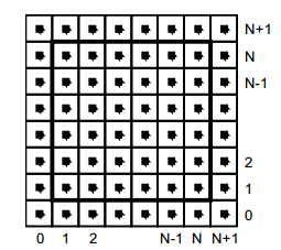
    We can think of fluids as a collection of cells or boxes (in 3D), each one interacting with it’s neighbor. Each cell has some basic properties like velocity and density and the transformation taking place in one cell is affecting the properties of neighbor cells (all of these happening million times per second).
    fluid-cells

    Being such a complex operation, computers (even the most powerful ones) can not simulate real time the fluid dynamics. For this we need to make some compromise. We’ll break the fluid up into a reasonable number of cells and try to do several interactions per second. That’s what Jos Stam’s approaching is doing great: sacrifice the fluid accuracy for a better visual presentation, more suitable for running real time. The best way to improve the simulation fluency is to reduce the solver iteration number. We’ll talk about this a little bit later.

    First we are staring by initializing some basic properties like the number of cells, the length of the timestamp, the amount of diffusion and viscosity etc. Also we need a density array and a velocity array and for each of them we set up a temporary array to switch the values between the new and old ones. This way we can store the old values while computing the new ones. Once we are done with the iteration we need to reset all the values to the default ones. For efficiency purposes we’ll use single dimensional array over double ones.

    The first step is to add some density to our cells:

    function addDensitySource(x, x0) {                
    	var size = self.numCells;        
    	while(size-- > -1) {
    		x[size] += _dt * x0[size];
    	}
    }

    then to add some velocity:

    FSolver.prototype.addCellVelocity = function() {
    	var size = self.numCells;
    	while(size-- > -1) {
    		if (isNaN(self.u[size])) continue;
    		self.u[size] += _dt * self.uOld[size];
    		if (isNaN(self.v[size])) continue;
    		self.v[size] += _dt * self.vOld[size];
    	}
    }

    Because some of the functions needs to be accessible only from main script i separated the internal (private) functions from the external (public) functions. But because Javascript is a prototypical language i used the object prototype method to extend it. That’s why some of the methods are declared with prototype and others as simple functions. However these aren’t accessible from the outside of FS namespace, which is declared as a global namespace. For this technique please see this great article Learning JavaScript Design Patterns.

    The process

    The basic structure of our solver is as follows. We start with some initial state for the velocity and the density and then update its values according to events happening in the environment.
    In our prototype we let the user apply forces and add density sources with the mouse (or we can extend this to touching devices too). There are many other possibilities this can be extended.

    Basically to simulate the fluid dynamics we need to familiarize our self with three main operations:

    Diffusion:

    Diffusion is the process when – in our case – the liquids doesn’t stay still, but are spreading out. Through diffusion each cell exchanges density with its direct neighbors. The array for the density is filled in from the user’s mouse movement. The cell’s density will decrease by losing density to its neighbors, but will also increase due to densities flowing in from the neighbors.

    Projection:

    This means the amount of fluid going in has to be exactly equal with the amount of fluid going out, otherwise may happens that the net inflow in some cells to be higher or lower than the net inflow of the neighbor cells. This may cause the simulation to react completely chaotic. This operation runs through all the cells and fixes them up to maintain in equilibrium.

    Advection:

    The key idea behind advection is that moving densities would be easy to solve if the density were modeled as a set of particles. In this case we would simply have to trace the particles though the velocity field. For example, we could pretend that each grid cell’s center is a particle and trace it through the velocity field. So advection in fact is a velocity applied to each grid cell. This is what makes things move.

    setBoundary():

    We assume that the fluid is contained in a box with solid walls: no flow should exit the walls. This simply means that the horizontal component of the velocity should be zero on the vertical walls, while the vertical component of the velocity should be zero on the horizontal walls. So in fact every velocity in the layer next to the outer layer is mirrored. The following code checks the boundaries of fluid cells.

    function setBoundary(bound, x) {
    	var dst1, dst2, src1, src2, i;
    	var step = FLUID_IX(0, 1) - FLUID_IX(0, 0);
    	dst1 = FLUID_IX(0, 1);
    	src1 = FLUID_IX(1, 1);
    	dst2 = FLUID_IX(_NX+1, 1);
    	src2 = FLUID_IX(_NX, 1);
    
    	if (wrap_x) {
    		src1 ^= src2;
    		src2 ^= src1;
    		src1 ^= src2;
    	}
    
    	if (bound == 1 && !wrap_x) {
    		for (i = _NY; i > 0; --i) {
    			x[dst1] = -x[src1]; dst1 += step; src1 += step;
    			x[dst2] = -x[src2]; dst2 += step; src2 += step;
    		}
    	} else {
    		for (i = _NY; i > 0; --i) {
    			x[dst1] = x[src1]; dst1 += step; src1 += step;
    			x[dst2] = x[src2]; dst2 += step; src2 += step;
    		}
    	}
    
    	dst1 = FLUID_IX(1, 0);
    	src1 = FLUID_IX(1, 1);
    	dst2 = FLUID_IX(1, _NY+1);
    	src2 = FLUID_IX(1, _NY);
    
    	if (wrap_y) {
    		src1 ^= src2;
    		src2 ^= src1;
    		src1 ^= src2;
    	}
    
    	if (bound == 2 && !wrap_y) {
    		for (i = _NX; i > 0 ; --i) {
    			x[dst1++] = -x[src1++];
    			x[dst2++] = -x[src2++];
    		}
    	} else {
    		for (i = _NX; i > 0; --i) {
    			x[dst1++] = x[src1++];
    			x[dst2++] = x[src2++];
    		}
    	}
    
    	x[FLUID_IX(0, 0)] = .5 * (x[FLUID_IX(1, 0)] + x[FLUID_IX(0, 1)]);
    	x[FLUID_IX(0, _NY+1)] = .5 * (x[FLUID_IX(1, _NY+1)] + x[FLUID_IX(0, _NY)]);
    	x[FLUID_IX(_NX+1, 0)] = .5 * (x[FLUID_IX(_NX, 0)] + x[FLUID_IX(_NX+1, _NX)]);
    	x[FLUID_IX(_NX+1, _NY+1)] = .5 * (x[FLUID_IX(_NX, _NY+1)] + x[FLUID_IX(_NX+1, _NY)]);
    }

    The main simulation function is implemented as follow:

    FSolver.prototype.updateDensity = function() {        
    	addDensitySource(this.density, this.densityOld);
    
    	if (_doVorticityConfinement) {            
    		calcVorticityConfinement(this.uOld, this.vOld);            
    	}
    
    	diffuse(0, this.densityOld, this.density, 0);
    	advect(0, this.density, this.densityOld, this.u, this.v);
    }
    
    FSolver.prototype.updateVelocity = function() {
    	this.addCellVelocity();
    	this.SWAP('uOld', 'u');
    	diffuse(1, this.u, this.uOld, _visc);
    	this.SWAP('vOld', 'v');        
    	diffuse(2, this.v, this.vOld, _visc);        
    	project(this.u, this.v, this.uOld, this.vOld);
    
    	this.SWAP('uOld', 'u');
    	this.SWAP('vOld', 'v');
    	advect(1, this.u, this.uOld, this.uOld, this.vOld);
    	advect(2, this.v, this.vOld, this.uOld, this.vOld);
    	project(this.u, this.v, this.uOld, this.vOld);
    }

    We are calling these functions on each frame on the main drawing method. For rendering the cells i used canvas putImageData() method which accepts as parameter an image data, whose values are in fact the fluid solver values obtained from the density array. My first attempt was to generate a particle field, associate to each particle density, velocity etc. (so all the data necessarily making a fluid simulation), connect each particle in a single linked list, knowing this is a much faster method for constructing an array, instead using the traditional one. Then using a fast and efficient method to trace a line, best known as Extremely Fast Line Algorithm or Xiaolin Wu’s line algorithm with anti aliasing (http://www.bytearray.org/?p=67) i thought i could gain more FPS for a smoother animation, but turned out being a very buggy implementation, so for the moment i abandoned the idea, but i will revised once i will have more time. Anyway i don’t swipe out this code part. You can find some utility functions too for my attempting, like implementing the AS3 Bitmap and BitmapData classes.

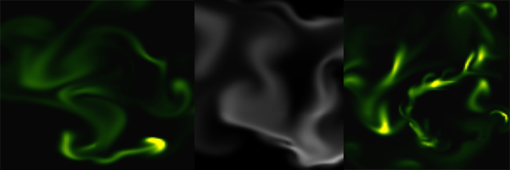
    And here is the monochrome version:
    www.esimov.com/experiments/javascript/fluid-solver-mono/

    The simulation is fully adapted to touch devices, but i think you need a really powerful device to run the fluid simulation decently.

    What’s next?

    That’s all. Hopefully this will be a solid base to explore further this field and add some extra functionality.

  • Cloth simulation with RK4 numerical integration

    Cloth simulation with RK4 numerical integration

    Click here to see it in action

    (click to see it in action)

    In this article I will discuss about something which is best known as numerical integration. I have always been fascinated by the cloth simulations, and wondered how it can be possible to reproduce this visually appealing effect using Actionscript, knowing that the AVM (Adobe Virtual Machine) is lacking well behind other languages like Java, not to mention C++ in terms of pure computation performance. Well to my surprise, after implementation I managed to obtain a pretty solid frame rate.

    The concept

    The core algorithm of the simulation is based on two concept known in physics as the Newton law’s of motion and restoration of force. This method is reasonably simple and robust and is a good general candidate for numerical solution of differential equations when combined with an intelligent adaptive step-size routine. After surfing the net for some tips and inspiration and reading Keith Peter’s book (AdvancED ActionScript 3.0 Animation), I got a grasp about the whole concept and physics acting behind it.

    The last temptation to implement my version came when I saw this amazing experiment implemented in Processing.

    The backbone of every clothing simulation is the so called numerical integration. There are many different techniques and implementation for physics simulation but, most of them use one of the three widespread integration method: Euler integration, Verlet integration and Runge-Kutta. The most significant difference between these methods consist in the accuracy of the movement.

    The Euler integration is the simplest one and uses the following algorithm: first calculate the actual position of the object, concatenate by the velocity and then apply acceleration. This is a very straightforward approximation with a very good performance, only it’s not accurate (unless we use an extremely small timestep size  – which we have no control over).

    The Verlet integration is very similar with Euler integration only this time we’ll get rid of the velocity component. We only need to calculate the change in position applying the acceleration value (A = F/m) which is a scalar component (the position and velocity actually are vectors). This is however velocity. So knowing the previous position and acceleration we could calculate the current position at the next frame. Keith Peters explain the differences between implementations in a very fashionable and enjoyable manner, so you should understand it easily. However my implementation differs quite enough from that one used in Keith’s book.

    Click to image

    (click to see it in action)

    The implementation

    In this experiment i’m gonna use Runge Kutta or simply RK4 implementation, but we can implement almost with the same accuracy the Verlet integration too. Very simply put, the algorithm first calculate the position and velocity at a certain interval (this calculation is done 4 times) and then make an approximation of them, and the average should be the object position and velocity at a certain position in time. The strength of this method is it’s accuracy, considering the minimal performance loss (i got almost constant 60 fps on my machine).

    Translated to AS3 it looks like this:

    /**
     * Get initial position, K1 velocity
     * apply forces and velocity, the result is K2
     */
    
    for (i = 0; i < numPart; i++)
    {
    	p = particles[i];
    
    	if (!p.fixed)
    	{
    		originalPos = originalPosV[i];
    		k1Vel = k1VelV[i];
    
    		s = (0.5 * t);
    		k1Vel.x *= s;
    		k1Vel.y *= s;
    		k1Vel.z *= s;
    		p.position.x = originalPos.x + k1Vel.x;
    		p.position.y = originalPos.y + k1Vel.y;
    		p.position.z = originalPos.z + k1Vel.z;
    
    		originalVel = originalVelV[i];
    		k1Force = k1ForceV[i];
    
    		s = (0.5 * t / p.mass);
    		k1Force.x *= s;
    		k1Force.y *= s;
    		k1Force.z *= s;
    		p.velocity.x = originalVel.x + k1Force.x;
    		p.velocity.y = originalVel.y + k1Force.y;
    		p.velocity.z = originalVel.z + k1Force.z;
    	}
    }
    
    particleSystem.applyForces();
    
    for (i = 0; i < numPart; i++)
    {
    	p = particles[i];
    
    	if (!p.fixed)
    	{
    		k2ForceV[i].x = p.force.x;
    		k2ForceV[i].y = p.force.y;
    		k2ForceV[i].z = p.force.z;
    		k2VelV[i].x = p.velocity.x;
    		k2VelV[i].y = p.velocity.y;
    		k2VelV[i].z = p.velocity.z;
    	}
    
    	p.force.x = 0;
    	p.force.y = 0;
    	p.force.z = 0;
    }
    
    /**
     * Get initial position, K2 velocity
     * apply forces and velocity, the result is K3
     */
    
    for (i = 0; i < numPart; i++)
    {
    	p = particles[i];
    
    	if (!p.fixed)
    	{
    		originalPos = originalPosV[i];
    		k2Vel = k2VelV[i];
    
    		s = (0.5 * t);
    		k2Vel.x *= s;
    		k2Vel.y *= s;
    		k2Vel.z *= s;
    		p.position.x = originalPos.x + k2Vel.x;
    		p.position.y = originalPos.y + k2Vel.y;
    		p.position.z = originalPos.z + k2Vel.z;
    
    		originalVel = originalVelV[i];
    		k2Force = k2ForceV[i];
    
    		s = (0.5 * t / p.mass);
    		k2Force.x *= s;
    		k2Force.y *= s;
    		k2Force.z *= s;
    		p.velocity.x = originalVel.x + k2Force.x;
    		p.velocity.y = originalVel.y + k2Force.y;
    		p.velocity.z = originalVel.z + k2Force.z;
    	}
    }
    
    particleSystem.applyForces();
    
    for (i = 0; i < numPart; i++)
    {
    	p = particles[i];
    
    	if (!p.fixed)
    	{
    		k3ForceV[i].x = p.force.x;
    		k3ForceV[i].y = p.force.y;
    		k3ForceV[i].z = p.force.z;
    		k3VelV[i].x = p.velocity.x;
    		k3VelV[i].y = p.velocity.y;
    		k3VelV[i].z = p.velocity.z;
    	}
    
    	p.force.x = 0;
    	p.force.y = 0;
    	p.force.z = 0;
    }
    
    /**
     * Get initial position, K3 velocity
     * apply forces and velocity, the result is K4
     */
    
    for (i = 0; i < numPart; i++)
    {
    	p = particles[i];
    
    	if (!p.fixed)
    	{
    		originalPos = originalPosV[i];
    		k3Vel = k3VelV[i];
    
    		s = (0.5 * t);
    		k3Vel.x *= s;
    		k3Vel.y *= s;
    		k3Vel.z *= s;
    		p.position.x = originalPos.x + k2Vel.x;
    		p.position.y = originalPos.y + k2Vel.y;
    		p.position.z = originalPos.z + k2Vel.z;
    
    		originalVel = originalVelV[i];
    		k3Force = k3ForceV[i];
    
    		s = (0.5 * t / p.mass);
    		k3Force.x *= s;
    		k3Force.y *= s;
    		k3Force.z *= s;
    		p.velocity.x = originalVel.x + k3Force.x;
    		p.velocity.y = originalVel.y + k3Force.y;
    		p.velocity.z = originalVel.z + k3Force.z;
    	}
    }
    
    particleSystem.applyForces();
    
    for (i = 0; i < numPart; i++)
    {
    	p = particles[i];
    
    	if (!p.fixed)
    	{
    		k4ForceV[i].x = p.force.x;
    		k4ForceV[i].y = p.force.y;
    		k4ForceV[i].z = p.force.z;
    		k4VelV[i].x = p.velocity.x;
    		k4VelV[i].y = p.velocity.y;
    		k4VelV[i].z = p.velocity.z;
    	}
    
    	p.force.x = 0;
    	p.force.y = 0;
    	p.force.z = 0;
    }
    
    /**
     * Update initial position and velocity based on intermediate values
     */
    
    for (i = 0; i < numPart; i++)
    {
    	p = particles[i];
    
    	if (!p.fixed)
    	{
    		//position
    
    		originalPos = originalPosV[i];
    		k1Vel = k1VelV[i];
    		k2Vel = k2VelV[i];
    		k3Vel = k3VelV[i];
    		k4Vel = k4VelV[i];
    
    		k2VelInt.x = k2Vel.x;
    		k2VelInt.y = k2Vel.y;
    		k2VelInt.z = k2Vel.z;
    		s = (2);
    		k2VelInt.x *= s;
    		k2VelInt.y *= s;
    		k2VelInt.z *= s;
    
    		k3VelInt.x = k3Vel.x;
    		k3VelInt.y = k3Vel.y;
    		k3VelInt.z = k3Vel.z;
    		s = (2);
    		k3VelInt.x *= s;
    		k3VelInt.y *= s;
    		k3VelInt.z *= s;
    
    		intVel.x = k1Vel.x + k2Vel.x + k3Vel.x + k4Vel.x;
    		intVel.y = k1Vel.y + k2Vel.y + k3Vel.y + k4Vel.y;
    		intVel.z = k1Vel.z + k2Vel.z + k3Vel.z + k4Vel.z;
    		s = (t / 6);
    		intVel.x *= s;
    		intVel.y *= s;
    		intVel.z *= s;
    		p.position.x = originalPos.x + intVel.x;
    		p.position.y = originalPos.y + intVel.y;
    		p.position.z = originalPos.z + intVel.z;
    
    		// velocity
    
    		originalVel = originalVelV[i];
    		k1Force = k1ForceV[i];
    		k2Force = k2ForceV[i];
    		k3Force = k3ForceV[i];
    		k4Force = k4ForceV[i];
    
    		k2ForceInt.x = k2Force.x;
    		k2ForceInt.y = k2Force.y;
    		k2ForceInt.z = k2Force.z;
    		s = (2);
    		k2ForceInt.x *= s;
    		k2ForceInt.y *= s;
    		k2ForceInt.z *= s;
    
    		k3ForceInt.x = k3Force.x;
    		k3ForceInt.y = k3Force.y;
    		k3ForceInt.z = k3Force.z;
    		s = (2);
    		k3ForceInt.x *= s;
    		k3ForceInt.y *= s;
    		k3ForceInt.z *= s;
    
    		intForce.x = k1Force.x + k2Force.x + k3Force.x + k4Force.x;
    		intForce.y = k1Force.y + k2Force.y + k3Force.y + k4Force.y;
    		intForce.z = k1Force.z + k2Force.z + k3Force.z + k4Force.z;
    		s = (t / 6 * p.mass);
    		intForce.x *= s;
    		intForce.y *= s;
    		intForce.z *= s;
    		p.velocity.x = originalVel.x + intForce.x;
    		p.velocity.y = originalVel.y + intForce.y;
    		p.velocity.z = originalVel.z + intForce.z;
    	}
    }

    (For a comparison between different numerical integration methods read this article: http://codeflow.org/entries/2010/aug/28/integration-by-example-euler-vs-verlet-vs-runge-kutta/.)

    Here is the final result (press space to show/hide the stats).

    Press right arrow to show wire frame and texture simultaneously, up arrow to show only bitmap texture and left arrow to show only the wire-frame.