Category: HTML5

  • Perlin noise based Minecraft rendering experiment

    Perlin noise based Minecraft rendering experiment

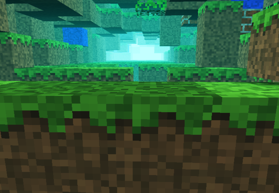
    Recently i was involved in a few different commercial projects, was toying with Golang, the shiny new language from Google and made some small snippets to test the language capability (i put them in my gist repository). In conclusion i somehow completely missed the creative coding. I had a few ideas and conceptions which i wanted to realize at an earlier or later stage. One of them was to adapt Notch minecraft renderer to be used in combination with perlin or simplex noise for generating random rendering maps.

    minecraft

    For that reason i ported to Javascript the original perlin noise algorithm written in Java. You can find the code here: https://gist.github.com/esimov/586a439f53f62f67083e. I won’t go into much details of how the perlin noise algorithm is working, if you are interested you can find a well explained paper here: http://webstaff.itn.liu.se/~stegu/simplexnoise/simplexnoise.pdf.

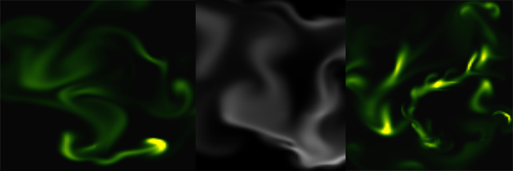
    As a starting point I put together a small experiment creating randomly generated perlin noise maps, and testing the granularity and dispersion of randomly selected seeding points to see how much they can be customized to create different noise patterns. I’m honest, actually these maps are not 100% randomly distributed, although they can be randomly seeded too, but for our scope I used a pretty neat algorithm for uniform granularity:

    
    // Seeded random number generator
    function seed(x) {
        x = (x<<13) ^ x;
        return ( 1.0 - ( (x * (x * x * 15731 + 789221) + 1376312589) & 0x7fffffff) / 1073741824.0);
    }
    

    And here is the working example:

    See the Pen Perlin metaball by Endre Simo (@esimov) on CodePen.

    The question that may arise: why should we need the perlin noise “thing” to generate different minecraft styled procedural terrain map? By generating randomly distributed noise we can further adjust the color mapping, then extract some of the areas above or below to certain values, which at a later state we can combine or even integrate into the core map generation logic. If you look at the alchemy behind the code responsible for programatically generating the terrain blocks, you will soon realize that we have all the ingredients (by manipulating some pixels here and there) to integrate the noise map into the block generation algorithm.

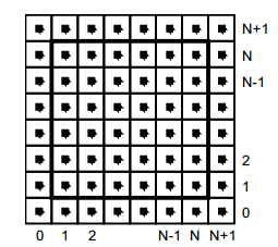
    In InitMap function we populate the map array with some initial values, then at a later stage after we generate the noise map, we extract the data as follows:

    
    for (var cell = 0; cell < pixels.length; cell += 4) {
        var ii = Math.floor(cell/4);
        var x = ii % canvasWidth;
        var y = Math.floor(ii / canvasWidth);
        var xx = 123 + x * .02;
        var yy = 324 + y * .02;
        
        var value = Math.floor((perlin.noise(xx,yy,1))*256);              
        pixels[cell] = pixels[cell + 1] = pixels[cell + 2] = value;
        pixels[cell + 3] = 255; // alpha.
    }
    

    then we go through the pixels data, setting up the condition on which data should be processed. In our actual case if the pixel color extracted is below to some certain value (this values are actually values extracted from the perlin noise map) then we set the map data to 0. This is why the perlin noise seed granularity is important. As smoother the transition between points is, as subtle would be the map generated.

    
    if ((pixelCol & 0xff * 0.48) < (64 - y) << 2) {
        map[i] = 0;
    }
    

    This is the basic logic for generating random minecraft terrain. We can even adjust the seed offset in perlin noise script to generate different patterns, however in my experiment seems that this doesn’t matter to much.

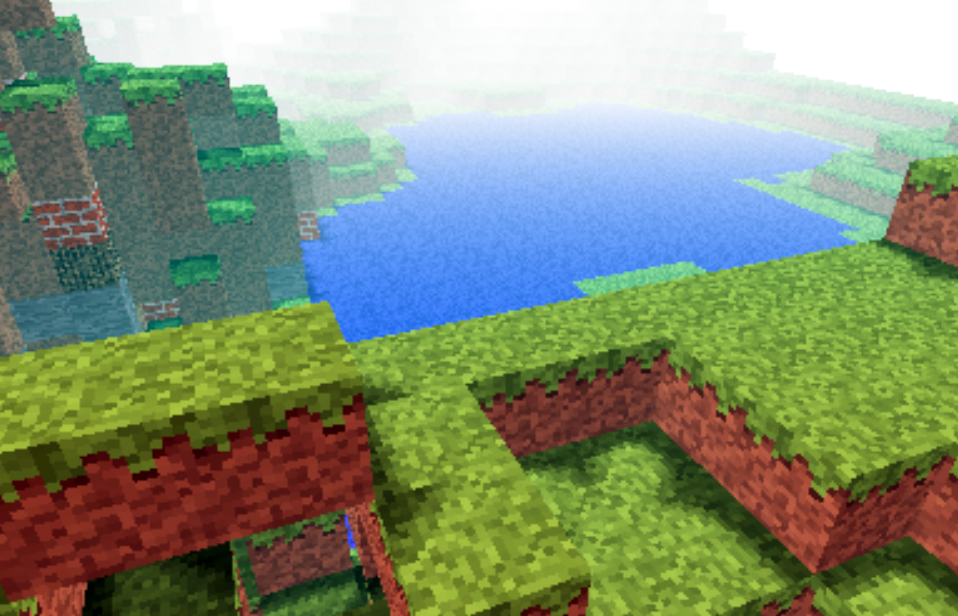
    The rendering engine is based on notch code, however i made some optimization adding some fake shadows and distance fog, creating a more ambiental environment.

    This is the code which creates the distance fog effect:

    
    var r = ((col >> 16) & 0xff) * br * ddist / (255 * 255);
    var g = ((col >> 8) & 0xff) * br * ddist / (255 * 255);
    var b = ((col) & 0xff) * br * ddist / (255 * 255);
    
    if(ddist <= 155) r += 155-ddist;
    if(ddist <= 255) g += 255-ddist;
    if(ddist <= 255) b += 255-ddist;  
    
    pixels[(x + y * w) * 4 + 0] = r;
    pixels[(x + y * w) * 4 + 1] = g;
    pixels[(x + y * w) * 4 + 2] = b;
    

    Playing with values i discovered that actually i can “move the camera around the scene” (actually here we have a fictive camera, meaning that not the camera is moving around scene, but the objects are projected around some fictive coordinates), so it was quite easy to get the mouse position and adjust the camera relative to the mouse position, this way including some user interaction into the scene.

    Version 2

    Even tough the desired effect pretty much satisfied my expectations, something was really missing from the original version: it was not possible to generate randomly seeded terrain maps and also the generated map was pretty much the same. So I have extended the first version with random map generation, replaced the Perlin noise generator with the simplex noise, added fake shadow and fog to give the feeling of depth and on top of these i have also included a control panel to play with the values. This is how it came out:

    The source code can be found on my Github page:

    https://github.com/esimov/minecraft.js

  • Navier Stokes Fluid Simulation on HTML5 Canvas

    Navier Stokes Fluid Simulation on HTML5 Canvas

    Implementing real time fluid simulation in pure Javascript was a long desire of me and has been sitting in my todo list from a long time on. However from various reasons i never found enough time to start working on it. I know it’s nothing new and there are quite a few implementations done on canvas already (maybe the best known is this: http://nerget.com/fluidSim/), but i wanted to do mine without to relay to others work and to use the core logic as found on the original paper.

    For me one of the most inspiring real-time 2D fluid simulations based on Navier Stokes equations was that created by Memo Akten, originally implemented in Processing (a Java based programming language, very suitable for digital artists for visual experimentation), lately ported to OpenFrameworks (a C++ framework) then implemented in AS 3.0 by Eugene Zatepyakin http://blog.inspirit.ru/?p=248.

    The code is based on Jos Stam’s famous paper – Real-Time Fluid Dynamics for Games, but another useful resource which i found during preparation and development was a paper from Mike Ash: Fluid Simulation for Dummies. As the title suggest, the concept is explained very clearly even if the equations behind are quite complex, which means without a good background in physics and differential equations it’s difficult to understand. This does not means that i’m a little genius in maths or physics :). In this post i will sketch briefly some of the main concepts behind the theory and more importantly how can be implemented in Javascript. As a side note, this simulation does not take advantages of the GPU power, so it’s not running on WebGL. For a WebGL implementation see http://www.ibiblio.org/e-notes/webgl/gpu/fluid.htm.

    fluid-solvers

    The basic concept

    We can think of fluids as a collection of cells or boxes (in 3D), each one interacting with it’s neighbor. Each cell has some basic properties like velocity and density and the transformation taking place in one cell is affecting the properties of neighbor cells (all of these happening million times per second).
    fluid-cells

    Being such a complex operation, computers (even the most powerful ones) can not simulate real time the fluid dynamics. For this we need to make some compromise. We’ll break the fluid up into a reasonable number of cells and try to do several interactions per second. That’s what Jos Stam’s approaching is doing great: sacrifice the fluid accuracy for a better visual presentation, more suitable for running real time. The best way to improve the simulation fluency is to reduce the solver iteration number. We’ll talk about this a little bit later.

    First we are staring by initializing some basic properties like the number of cells, the length of the timestamp, the amount of diffusion and viscosity etc. Also we need a density array and a velocity array and for each of them we set up a temporary array to switch the values between the new and old ones. This way we can store the old values while computing the new ones. Once we are done with the iteration we need to reset all the values to the default ones. For efficiency purposes we’ll use single dimensional array over double ones.

    The first step is to add some density to our cells:

    function addDensitySource(x, x0) {                
    	var size = self.numCells;        
    	while(size-- > -1) {
    		x[size] += _dt * x0[size];
    	}
    }

    then to add some velocity:

    FSolver.prototype.addCellVelocity = function() {
    	var size = self.numCells;
    	while(size-- > -1) {
    		if (isNaN(self.u[size])) continue;
    		self.u[size] += _dt * self.uOld[size];
    		if (isNaN(self.v[size])) continue;
    		self.v[size] += _dt * self.vOld[size];
    	}
    }

    Because some of the functions needs to be accessible only from main script i separated the internal (private) functions from the external (public) functions. But because Javascript is a prototypical language i used the object prototype method to extend it. That’s why some of the methods are declared with prototype and others as simple functions. However these aren’t accessible from the outside of FS namespace, which is declared as a global namespace. For this technique please see this great article Learning JavaScript Design Patterns.

    The process

    The basic structure of our solver is as follows. We start with some initial state for the velocity and the density and then update its values according to events happening in the environment.
    In our prototype we let the user apply forces and add density sources with the mouse (or we can extend this to touching devices too). There are many other possibilities this can be extended.

    Basically to simulate the fluid dynamics we need to familiarize our self with three main operations:

    Diffusion:

    Diffusion is the process when – in our case – the liquids doesn’t stay still, but are spreading out. Through diffusion each cell exchanges density with its direct neighbors. The array for the density is filled in from the user’s mouse movement. The cell’s density will decrease by losing density to its neighbors, but will also increase due to densities flowing in from the neighbors.

    Projection:

    This means the amount of fluid going in has to be exactly equal with the amount of fluid going out, otherwise may happens that the net inflow in some cells to be higher or lower than the net inflow of the neighbor cells. This may cause the simulation to react completely chaotic. This operation runs through all the cells and fixes them up to maintain in equilibrium.

    Advection:

    The key idea behind advection is that moving densities would be easy to solve if the density were modeled as a set of particles. In this case we would simply have to trace the particles though the velocity field. For example, we could pretend that each grid cell’s center is a particle and trace it through the velocity field. So advection in fact is a velocity applied to each grid cell. This is what makes things move.

    setBoundary():

    We assume that the fluid is contained in a box with solid walls: no flow should exit the walls. This simply means that the horizontal component of the velocity should be zero on the vertical walls, while the vertical component of the velocity should be zero on the horizontal walls. So in fact every velocity in the layer next to the outer layer is mirrored. The following code checks the boundaries of fluid cells.

    function setBoundary(bound, x) {
    	var dst1, dst2, src1, src2, i;
    	var step = FLUID_IX(0, 1) - FLUID_IX(0, 0);
    	dst1 = FLUID_IX(0, 1);
    	src1 = FLUID_IX(1, 1);
    	dst2 = FLUID_IX(_NX+1, 1);
    	src2 = FLUID_IX(_NX, 1);
    
    	if (wrap_x) {
    		src1 ^= src2;
    		src2 ^= src1;
    		src1 ^= src2;
    	}
    
    	if (bound == 1 && !wrap_x) {
    		for (i = _NY; i > 0; --i) {
    			x[dst1] = -x[src1]; dst1 += step; src1 += step;
    			x[dst2] = -x[src2]; dst2 += step; src2 += step;
    		}
    	} else {
    		for (i = _NY; i > 0; --i) {
    			x[dst1] = x[src1]; dst1 += step; src1 += step;
    			x[dst2] = x[src2]; dst2 += step; src2 += step;
    		}
    	}
    
    	dst1 = FLUID_IX(1, 0);
    	src1 = FLUID_IX(1, 1);
    	dst2 = FLUID_IX(1, _NY+1);
    	src2 = FLUID_IX(1, _NY);
    
    	if (wrap_y) {
    		src1 ^= src2;
    		src2 ^= src1;
    		src1 ^= src2;
    	}
    
    	if (bound == 2 && !wrap_y) {
    		for (i = _NX; i > 0 ; --i) {
    			x[dst1++] = -x[src1++];
    			x[dst2++] = -x[src2++];
    		}
    	} else {
    		for (i = _NX; i > 0; --i) {
    			x[dst1++] = x[src1++];
    			x[dst2++] = x[src2++];
    		}
    	}
    
    	x[FLUID_IX(0, 0)] = .5 * (x[FLUID_IX(1, 0)] + x[FLUID_IX(0, 1)]);
    	x[FLUID_IX(0, _NY+1)] = .5 * (x[FLUID_IX(1, _NY+1)] + x[FLUID_IX(0, _NY)]);
    	x[FLUID_IX(_NX+1, 0)] = .5 * (x[FLUID_IX(_NX, 0)] + x[FLUID_IX(_NX+1, _NX)]);
    	x[FLUID_IX(_NX+1, _NY+1)] = .5 * (x[FLUID_IX(_NX, _NY+1)] + x[FLUID_IX(_NX+1, _NY)]);
    }

    The main simulation function is implemented as follow:

    FSolver.prototype.updateDensity = function() {        
    	addDensitySource(this.density, this.densityOld);
    
    	if (_doVorticityConfinement) {            
    		calcVorticityConfinement(this.uOld, this.vOld);            
    	}
    
    	diffuse(0, this.densityOld, this.density, 0);
    	advect(0, this.density, this.densityOld, this.u, this.v);
    }
    
    FSolver.prototype.updateVelocity = function() {
    	this.addCellVelocity();
    	this.SWAP('uOld', 'u');
    	diffuse(1, this.u, this.uOld, _visc);
    	this.SWAP('vOld', 'v');        
    	diffuse(2, this.v, this.vOld, _visc);        
    	project(this.u, this.v, this.uOld, this.vOld);
    
    	this.SWAP('uOld', 'u');
    	this.SWAP('vOld', 'v');
    	advect(1, this.u, this.uOld, this.uOld, this.vOld);
    	advect(2, this.v, this.vOld, this.uOld, this.vOld);
    	project(this.u, this.v, this.uOld, this.vOld);
    }

    We are calling these functions on each frame on the main drawing method. For rendering the cells i used canvas putImageData() method which accepts as parameter an image data, whose values are in fact the fluid solver values obtained from the density array. My first attempt was to generate a particle field, associate to each particle density, velocity etc. (so all the data necessarily making a fluid simulation), connect each particle in a single linked list, knowing this is a much faster method for constructing an array, instead using the traditional one. Then using a fast and efficient method to trace a line, best known as Extremely Fast Line Algorithm or Xiaolin Wu’s line algorithm with anti aliasing (http://www.bytearray.org/?p=67) i thought i could gain more FPS for a smoother animation, but turned out being a very buggy implementation, so for the moment i abandoned the idea, but i will revised once i will have more time. Anyway i don’t swipe out this code part. You can find some utility functions too for my attempting, like implementing the AS3 Bitmap and BitmapData classes.

    And here is the monochrome version:
    www.esimov.com/experiments/javascript/fluid-solver-mono/

    The simulation is fully adapted to touch devices, but i think you need a really powerful device to run the fluid simulation decently.

    What’s next?

    That’s all. Hopefully this will be a solid base to explore further this field and add some extra functionality.

  • A new look for my site

    A new look for my site

    It has been a very long time since my last post, ignoring almost any online social activity and not having too much free time for visual experimentation and self study, but finally find some time to finish the new look of my site. Actually is not only a new look, but a completely reworked and redesigned site from ground up. The previous version was based on WordPress. I liked the flexibility and easy to use feature of WordPress, which in essence could be to reduce to a two-step workflow: search for a theme, install it and you are good to go.

    footer-logo

    BTW this is the logo of my site designed by myself

    I was thinking from time to time, to give some personality to my site, meaning trying to keep myself distant from WP, maybe using only the backend part for content upload, post editing and any other content management activity.

    Searching for WP alternatives I found roots.io and Octopress the two most suitable alternatives for WordPress. Initially i opted for the first one only for the reason that i can preserve the current content without too much overhead. I found this a good alternative to WordPress for it’s minimal and accessible markup and for the fact it can rewrite the conventional wordpress URL’s, meaning it makes the path names cleaner, but on the other hand i thought it would be more challenging but at the same time more satisfying and rewarding to create my own custom Javascript library for building the site. For this scope i used PHP only for calling some web services, pulling out the content from WordPress database, wrapping as a JSON object, then transmitting over to the front end where with some ajax call i can build the whole page.

    I wanted to build the site using cutting edge modern web technologies for this reason many of the features are not working as expected on older browsers. The whole site has been build up around HTML5, Canvas and CSS3 spiced with a lot of Javascript. This is somehow a mini MVC framework, the model part being responsible for obtaining the JSON data from backend, the controller having as main role to communicate with the view and model (triggering the model and passing the results to the view the latter organizing the received data in a visual manner).

    Many of you may ask why i didn’t make it with more fashinable MV* frameworks like Backbone, Angular.js or Ember.js? My answer is: when i started this project i wasn’t very familiar with these technologies, i only heard about them, and once started i wanted to make it till the end. Maybe sometime i will think differently and will give it a try, but till then i’m pretty satisfied with the result. Of course there are some bugs which i have to address, like responsiveness, awkward page rendering when selecting a specific tag and associating the posts with these tags. Feel free to give any feedback be as good or bad.

    As you probably realized sometimes you are redirected to my other domain name (esimov.com). I’m not completely decided either to keep esimov.com or esimov.com as my main blogging platform, the first one having a more ‘business-ish’ feeling, on the other hand the last one suiting more for a personal blogging scope. I will decide later.