Category: Experiments

  • 404 page

    404 page

    During the setup of my site i decided to create a custom 404 page, inspired by this nice canvas experiment made by Hakim. I wanted the bubbles to be bursted by mouse click and to integrate the representative “404” text message, which i wanted to be reactive to the mouse and wave movement.

    So for that reason i’ve rewrite the code pretty much for my own purposes, plus i wanted to integrate some searching functions into my site. For this reason i was looking for a free php searching engine. I found sphider to be well acclaimed among users and developers, so i gave it a try. I managed to setup the search engine almost instantly, however the visual appearance have to be polished a little bit.

    A challenge for me was to integrate the text into the canvas considering I opted for a big bold character. I’ve tried the canvas native fillText function, but the text edges were very jaggy, so i decided to inject SVG code into the canvas, which looked like this:

    
    var data = "data:image/svg+xml," +
        "<svg xmlns='http://www.w3.org/2000/svg' width='400' height='400'>" +
        "<foreignObject width='100%' height='100%'>" +
            "<div xmlns='http://www.w3.org/1999/xhtml' style='font: bold 160px Myriad Pro, Arial, Helvetica, Arial, sans-serif'>" +
                "<span style='color:rgb(32,124,202); opacity: 0.8; -webkit-text-stroke-color: white; -webkit-text-stroke-width: 2px'>" + letters[pos] + "</span>" +
            "</div>" +
        "</foreignObject>" +
    "</svg>";
    

    As a last element I introduced a twitter feeder, which search for every word i define, and used Modernizr for a fallback for browsers which does not support canvas. Sorry IE.

  • Organic Turing Pattern

    Organic Turing Pattern

    In this post i will present an experiment which i did a few months earlier, but because lately i was pretty occupied with various job related activities and with setting up this new blog (transferring the old content to the new host – plus a lot of other stuff), i have no time to publish this new experiment. More about below, but until then a few words about the background, inspiration and some of the key challenge i have faced during this process.

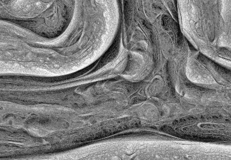
    This is an experiment inspired by a thoroughly explained article about the concept behind what is generally known as Turing Pattern. The Turing Patterns has become a key attraction in fact thanks to Jonathan McCabe popular paper Cyclic Symmetric Mutli-Scale Turing Patterns in which he explains the process behind the image generation algorithm like that one below, about what Frederik Vanhoutte know as W:blut wrote on his post:

    Quote leftIf you’ve seen any real­ity zoo/wild-life pro­gram you’ll rec­og­nize this. Five min­utes into the show you’re con­fronted with a wounded, mag­nif­i­cent ani­mal, held in cap­tiv­ity so its care­tak­ers can nur­ture and feed it. And inevitably, after three com­mer­cial breaks, they release it, teary-eyed, back into the wild. It’s a piv­otal moment that turns their leop­ard into anyone’s/no one’s leop­ard.Quote right

    That’s the feeling which emanates when you first see the organic like, somehow obscure (some may go even further and say: macabre or creepy) thing which is known as a Turing pattern. At first moment when you are confronted with it, some kind of emotion (be that fear or amazement or just a sight) is resurfaced. Definitely won’t let you neutral.

    This is the emotion which pushed me to try to implement it in Actionscript. (In parentheses be said this is not the best platform for computation intensive experiments.) Felix Woitzel did an amazing remake adaptation of the original pattern in WebGL. The performance with a good GPU is quite impressive. Maybe in the future i will try to port in WebGL. Anyway, there is another nice article by Jason Rampe, where he explains the algorithm of the Turing Pattern.

    So let’s face directly and dissect the core components of the algorithm.

    The basic concept

    The process is based on a series of different “turing” scales. Each scale has different values for activator, inhibitor, radius, amount and levels. We use a two dimensional grid which will be the basic container for activator, inhibitor and variations, all of them going to be of typed arrays (in our case Vectors.<>). At the first phase we will initialize the grid with random points between -1 and 1. In the next step we have to determine the shape of the pattern. For this case w’ll use a formula defined by the following method:

    for (var i:int = 0; i < levels; i++)
    {
    	var radius:int = int(Math.pow(base, i));
    	_radii[i] = radius;
    	_stepSizes[i] = Math.log(radius) * stepScale + stepOffset;
    }

    During each step of simulation we have to execute the following methods:

    1. Populate the grid with pixels at random locations. I’m gonna use a linked list to store the pixels properties: positions and colors. We will loop through all the pixels, the number of pixels will be defined by the grid with x height dimension.
    2. Average each grid cell location over a circular radius specified by activator, then store the results in the activator array, multiplied by the weight.
    3. Average each grid cell location over a circular radius specified by inhibitor, then store the results in the activator array, multiplied by the weight.
    4. In the next step we need to calculate the absolute difference between the activator and inhibitor using the the following formula: variations = variations + abs(activator[x,y] - inhibitor[x,y])

    Once we have all the activator, inhibitor and variations values calculated for each grid cells we proceed with updating the grids as follows:

    1. Find which grid cell has the lowest variation value
    2. Once we found the lowest variation value we update the grid by the following formula:
    for (var l:Number = 0; l < levels - 1; l++)
    {
    	var radius:int = int(_radii[l]);
    	fastBlur(activator, inhibitor, _blurBuffer, WIDTH, HEIGHT, radius);
    
    	//calculates the absolute difference between activator and inhibitor
    
    	for (var i:int = 0; i < n; i++)
    	{
    		_variations[i] = activator[i] - inhibitor[i];
    		if (_variations[i] < 0)
    		{
    			_variations[i] = -_variations[i];
    		}
    	}
    
    	//if first level then set some initial values for bestLevel and bestVariation 
    	if (l == 0)
    	{
    		for (i = 0; i < n; i++)
    		{
    			_bestVariation[i] = _variations[i];
    			_bestLevel[i] = l;
    			_directions[i] = activator[i] > inhibitor[i];
    		}
    		activator = _diffRight;
    		inhibitor = _diffLeft;
    	}
    	else
    	{
    		for (i = 0; i < n; i++)
    		{
    			if (_variations[i] < _bestVariation[i])
    			{
    				_bestVariation[i] = _variations[i];
    				_bestLevel[i] = l;
    				_directions[i] = activator[i] > inhibitor[i];
    
    			}
    		}
    		var swap:Vector. = activator;
    		activator = inhibitor;
    		inhibitor = swap;
    	}
    }

    As a last step we should average the gap between the levels by performing a blur technique for a nicer transition. We blur the image sequentially in two steps: first we blur the image vertically then horizontally.

    The challenge

    The most challenging part was related to the unknown factor about how well gonna handle the AVM2 the intensive CPU calculation. Well as you may have guessed not too well, especially with very large bitmap dimension and a lot of pixels needed to be manipulated, plus the extra performance loss “gained” after the bluring operation.

    For some kind of compensation benefits (in terms of performance) i decided to populate the BitmapData with a chained loop using single linked list, plus typed arrays as generally known the Vector.<> arrays are much faster compared to the traditional array stacks. After a not too impressive performance, i wondered how can i even more optimize the code for a better overcome. I decided to give it a try to Alchemy, and Joa Ebert’s TDSI, a Java based Actionscript compiler, as by that time was commonly known a better choice over AVM. Unfortunately i didn’t get too many support and helpful articles about the implementation and as a consequence my attempt was a failure, which resulted in a quite buggy and ugly output. After too many attempts without the wishful result, i gave up.

    That’s all in big steps. You can grab the source code from here. Feel free to post your remarks.

    ps: Be prepared this experiment will burn your CPU. 🙂

  • Sound visualization

    Sound visualization

    Sound visualization is one thing which I was always fascinated by. I stumbled upon this small Javascript experiment and thought would be nice to reproduce it in Actionscript, adding some spicy extra addons like interaction and sounds reacting shapes. So I decided to implement in Actionscript. Actually it went very well, in fact i only retained the core algorithm. The core algorithm consist in just a few lines:

    private function createSurface(a:Number, z:Number):Point3D
    {
    	var r:Number = W/10;
    	var R:Number = W/3;
    	var b:Number = -10*Math.cos(a*5 + T);
    
    	return new Point3D(W/2 + (R*Math.cos(a) + r*Math.sin(z+2*T))/z + Math.cos(a)*b,
    							   H/2 + (R*Math.sin(a))/z + Math.sin(a)*b, Z);
    }
    
    private function drawQuad(a:Number, da:Number, z:Number, dz:Number):void
    {
    	var v:Array = [createSurface(a,z),
    				   createSurface(a+da,z),
    				   createSurface(a+da, z+dz),
    				   createSurface(a, z+dz)];
    
    	_points = new Vector.();
    	_stroke = new GraphicsStroke();
    	_stroke.thickness = 1;
    	_stroke.fill = new GraphicsSolidFill(0x102020,0.95);
    
    	_path = new GraphicsPath(new Vector.(), new Vector.());
    	_path.moveTo(Point3D(v[0]).x, Point3D(v[0]).y);
    
    	for (var i:Number = 0; i < v.length; i++)
    	{
    		_path.lineTo(Point3D(v[i]).x, Point3D(v[i]).y);
    	}
    	_background = new GraphicsSolidFill(0x663399, 0.95);
    }

    First we create some quads using sine and cosine, multiplying by the radius, which is given as a constant. Then we store these quads on an array, setting their positions by calling the GraphicsPath.lineTo method. These positions are updated each time we loop through on an EnterFrame event listener. The fancy things happens here, where we use a fog variable to apply the shading effect by tweaking some depth illusion.

    And this is how it looks after implementation. By the way this is a good example of how robust and fast are <IGraphicsData> and drawGraphicsData functions combined.

    (Move the mouse to change the color shading intensity)

    After implementing the basic structure I thought – following the suggestion of some of the active members of wonderfl community – it would be nice to add some extra feature like sound visualization. Initially this little effect consists of some sinusoidally  curvy movement modifying the color intensity by the mouse position. You can check the effect by clicking on the image above.

    I was pleasantly surprised by the smoothly frame rate of the effect, so as i mentioned earlier the next step was to implement the algorithm for sound visualization. Thanks to makc3d audio API it was an easy job to obtain some samples which later could be used for the funky disco effect following the rhythm of the sound. This simple API connects to BeatPort portal, and by providing an unique key we can select from a various music genres. I opted for dubstep only because the high variation of beats can produce a very differentiated transition (a next step could be to implement an interface for selecting the different music channel).

    This is another variation.

    Playing with the values we can obtain different visualization effects. For example scaling up the bass bit rate we can obtain a nice upscaled flowing ring or reducing the radius value we should obtain a perfect circular cube like in the example below.

    Definitely a GUI interface would have been a better choice for playing with values, but because i put together this experiment in almost two hours i didn’t take the effort to polish the code. Maybe in a future time.

    (Scroll the mouse to jump to the next track)

    You can grab the source code here!

  • Cloth simulation with RK4 numerical integration

    Cloth simulation with RK4 numerical integration

    Click here to see it in action

    (click to see it in action)

    In this article I will discuss about something which is best known as numerical integration. I have always been fascinated by the cloth simulations, and wondered how it can be possible to reproduce this visually appealing effect using Actionscript, knowing that the AVM (Adobe Virtual Machine) is lacking well behind other languages like Java, not to mention C++ in terms of pure computation performance. Well to my surprise, after implementation I managed to obtain a pretty solid frame rate.

    The concept

    The core algorithm of the simulation is based on two concept known in physics as the Newton law’s of motion and restoration of force. This method is reasonably simple and robust and is a good general candidate for numerical solution of differential equations when combined with an intelligent adaptive step-size routine. After surfing the net for some tips and inspiration and reading Keith Peter’s book (AdvancED ActionScript 3.0 Animation), I got a grasp about the whole concept and physics acting behind it.

    The last temptation to implement my version came when I saw this amazing experiment implemented in Processing.

    The backbone of every clothing simulation is the so called numerical integration. There are many different techniques and implementation for physics simulation but, most of them use one of the three widespread integration method: Euler integration, Verlet integration and Runge-Kutta. The most significant difference between these methods consist in the accuracy of the movement.

    The Euler integration is the simplest one and uses the following algorithm: first calculate the actual position of the object, concatenate by the velocity and then apply acceleration. This is a very straightforward approximation with a very good performance, only it’s not accurate (unless we use an extremely small timestep size  – which we have no control over).

    The Verlet integration is very similar with Euler integration only this time we’ll get rid of the velocity component. We only need to calculate the change in position applying the acceleration value (A = F/m) which is a scalar component (the position and velocity actually are vectors). This is however velocity. So knowing the previous position and acceleration we could calculate the current position at the next frame. Keith Peters explain the differences between implementations in a very fashionable and enjoyable manner, so you should understand it easily. However my implementation differs quite enough from that one used in Keith’s book.

    Click to image

    (click to see it in action)

    The implementation

    In this experiment i’m gonna use Runge Kutta or simply RK4 implementation, but we can implement almost with the same accuracy the Verlet integration too. Very simply put, the algorithm first calculate the position and velocity at a certain interval (this calculation is done 4 times) and then make an approximation of them, and the average should be the object position and velocity at a certain position in time. The strength of this method is it’s accuracy, considering the minimal performance loss (i got almost constant 60 fps on my machine).

    Translated to AS3 it looks like this:

    /**
     * Get initial position, K1 velocity
     * apply forces and velocity, the result is K2
     */
    
    for (i = 0; i < numPart; i++)
    {
    	p = particles[i];
    
    	if (!p.fixed)
    	{
    		originalPos = originalPosV[i];
    		k1Vel = k1VelV[i];
    
    		s = (0.5 * t);
    		k1Vel.x *= s;
    		k1Vel.y *= s;
    		k1Vel.z *= s;
    		p.position.x = originalPos.x + k1Vel.x;
    		p.position.y = originalPos.y + k1Vel.y;
    		p.position.z = originalPos.z + k1Vel.z;
    
    		originalVel = originalVelV[i];
    		k1Force = k1ForceV[i];
    
    		s = (0.5 * t / p.mass);
    		k1Force.x *= s;
    		k1Force.y *= s;
    		k1Force.z *= s;
    		p.velocity.x = originalVel.x + k1Force.x;
    		p.velocity.y = originalVel.y + k1Force.y;
    		p.velocity.z = originalVel.z + k1Force.z;
    	}
    }
    
    particleSystem.applyForces();
    
    for (i = 0; i < numPart; i++)
    {
    	p = particles[i];
    
    	if (!p.fixed)
    	{
    		k2ForceV[i].x = p.force.x;
    		k2ForceV[i].y = p.force.y;
    		k2ForceV[i].z = p.force.z;
    		k2VelV[i].x = p.velocity.x;
    		k2VelV[i].y = p.velocity.y;
    		k2VelV[i].z = p.velocity.z;
    	}
    
    	p.force.x = 0;
    	p.force.y = 0;
    	p.force.z = 0;
    }
    
    /**
     * Get initial position, K2 velocity
     * apply forces and velocity, the result is K3
     */
    
    for (i = 0; i < numPart; i++)
    {
    	p = particles[i];
    
    	if (!p.fixed)
    	{
    		originalPos = originalPosV[i];
    		k2Vel = k2VelV[i];
    
    		s = (0.5 * t);
    		k2Vel.x *= s;
    		k2Vel.y *= s;
    		k2Vel.z *= s;
    		p.position.x = originalPos.x + k2Vel.x;
    		p.position.y = originalPos.y + k2Vel.y;
    		p.position.z = originalPos.z + k2Vel.z;
    
    		originalVel = originalVelV[i];
    		k2Force = k2ForceV[i];
    
    		s = (0.5 * t / p.mass);
    		k2Force.x *= s;
    		k2Force.y *= s;
    		k2Force.z *= s;
    		p.velocity.x = originalVel.x + k2Force.x;
    		p.velocity.y = originalVel.y + k2Force.y;
    		p.velocity.z = originalVel.z + k2Force.z;
    	}
    }
    
    particleSystem.applyForces();
    
    for (i = 0; i < numPart; i++)
    {
    	p = particles[i];
    
    	if (!p.fixed)
    	{
    		k3ForceV[i].x = p.force.x;
    		k3ForceV[i].y = p.force.y;
    		k3ForceV[i].z = p.force.z;
    		k3VelV[i].x = p.velocity.x;
    		k3VelV[i].y = p.velocity.y;
    		k3VelV[i].z = p.velocity.z;
    	}
    
    	p.force.x = 0;
    	p.force.y = 0;
    	p.force.z = 0;
    }
    
    /**
     * Get initial position, K3 velocity
     * apply forces and velocity, the result is K4
     */
    
    for (i = 0; i < numPart; i++)
    {
    	p = particles[i];
    
    	if (!p.fixed)
    	{
    		originalPos = originalPosV[i];
    		k3Vel = k3VelV[i];
    
    		s = (0.5 * t);
    		k3Vel.x *= s;
    		k3Vel.y *= s;
    		k3Vel.z *= s;
    		p.position.x = originalPos.x + k2Vel.x;
    		p.position.y = originalPos.y + k2Vel.y;
    		p.position.z = originalPos.z + k2Vel.z;
    
    		originalVel = originalVelV[i];
    		k3Force = k3ForceV[i];
    
    		s = (0.5 * t / p.mass);
    		k3Force.x *= s;
    		k3Force.y *= s;
    		k3Force.z *= s;
    		p.velocity.x = originalVel.x + k3Force.x;
    		p.velocity.y = originalVel.y + k3Force.y;
    		p.velocity.z = originalVel.z + k3Force.z;
    	}
    }
    
    particleSystem.applyForces();
    
    for (i = 0; i < numPart; i++)
    {
    	p = particles[i];
    
    	if (!p.fixed)
    	{
    		k4ForceV[i].x = p.force.x;
    		k4ForceV[i].y = p.force.y;
    		k4ForceV[i].z = p.force.z;
    		k4VelV[i].x = p.velocity.x;
    		k4VelV[i].y = p.velocity.y;
    		k4VelV[i].z = p.velocity.z;
    	}
    
    	p.force.x = 0;
    	p.force.y = 0;
    	p.force.z = 0;
    }
    
    /**
     * Update initial position and velocity based on intermediate values
     */
    
    for (i = 0; i < numPart; i++)
    {
    	p = particles[i];
    
    	if (!p.fixed)
    	{
    		//position
    
    		originalPos = originalPosV[i];
    		k1Vel = k1VelV[i];
    		k2Vel = k2VelV[i];
    		k3Vel = k3VelV[i];
    		k4Vel = k4VelV[i];
    
    		k2VelInt.x = k2Vel.x;
    		k2VelInt.y = k2Vel.y;
    		k2VelInt.z = k2Vel.z;
    		s = (2);
    		k2VelInt.x *= s;
    		k2VelInt.y *= s;
    		k2VelInt.z *= s;
    
    		k3VelInt.x = k3Vel.x;
    		k3VelInt.y = k3Vel.y;
    		k3VelInt.z = k3Vel.z;
    		s = (2);
    		k3VelInt.x *= s;
    		k3VelInt.y *= s;
    		k3VelInt.z *= s;
    
    		intVel.x = k1Vel.x + k2Vel.x + k3Vel.x + k4Vel.x;
    		intVel.y = k1Vel.y + k2Vel.y + k3Vel.y + k4Vel.y;
    		intVel.z = k1Vel.z + k2Vel.z + k3Vel.z + k4Vel.z;
    		s = (t / 6);
    		intVel.x *= s;
    		intVel.y *= s;
    		intVel.z *= s;
    		p.position.x = originalPos.x + intVel.x;
    		p.position.y = originalPos.y + intVel.y;
    		p.position.z = originalPos.z + intVel.z;
    
    		// velocity
    
    		originalVel = originalVelV[i];
    		k1Force = k1ForceV[i];
    		k2Force = k2ForceV[i];
    		k3Force = k3ForceV[i];
    		k4Force = k4ForceV[i];
    
    		k2ForceInt.x = k2Force.x;
    		k2ForceInt.y = k2Force.y;
    		k2ForceInt.z = k2Force.z;
    		s = (2);
    		k2ForceInt.x *= s;
    		k2ForceInt.y *= s;
    		k2ForceInt.z *= s;
    
    		k3ForceInt.x = k3Force.x;
    		k3ForceInt.y = k3Force.y;
    		k3ForceInt.z = k3Force.z;
    		s = (2);
    		k3ForceInt.x *= s;
    		k3ForceInt.y *= s;
    		k3ForceInt.z *= s;
    
    		intForce.x = k1Force.x + k2Force.x + k3Force.x + k4Force.x;
    		intForce.y = k1Force.y + k2Force.y + k3Force.y + k4Force.y;
    		intForce.z = k1Force.z + k2Force.z + k3Force.z + k4Force.z;
    		s = (t / 6 * p.mass);
    		intForce.x *= s;
    		intForce.y *= s;
    		intForce.z *= s;
    		p.velocity.x = originalVel.x + intForce.x;
    		p.velocity.y = originalVel.y + intForce.y;
    		p.velocity.z = originalVel.z + intForce.z;
    	}
    }

    (For a comparison between different numerical integration methods read this article: http://codeflow.org/entries/2010/aug/28/integration-by-example-euler-vs-verlet-vs-runge-kutta/.)

    Here is the final result (press space to show/hide the stats).

    Press right arrow to show wire frame and texture simultaneously, up arrow to show only bitmap texture and left arrow to show only the wire-frame.