Category: Tutorials

In this blog post i want to share my first impression about Typescript, the new programming language from Microsoft.

The background

Coming from Flash/Actionscript, and having done almost all my experiments in AS3, facing the loose typing nature of JavaScript was a bit daunting for me. Over the time I got familiarized myself with all the mystical parts of JavaScript, with it’s prototyping nature, with the strange fact that JS hasn’t a type interface, and you can declare a variable without declaring the type of that variable. In fact all the declared variables can take any type of value, and assigning a different type of value to the variable wont make the compiler to trow an exception (only if we force to do so). This proved to be the weakness of JavaScript and the most acclaimed factor which stand in front of developing highly scalable applications.

wo

The first question that may arise is what is Typescript? The answer is: Typescript is a superset of JavaScript which compiles to JavaScript at runtime, all while maintaining your existing code and using the existing libraries. And why Typescript? The short answer: because Typescript is awesome. The long answer will follow.

One of the main benefits using typescript is code validation at compile time and compilation to native Javascript file at the runtime.

This differentiate Typescript from other competitors, nominating mainly two contenders: DART ( which is a very heavy assault initiative from Google meant to eliminate all the weakness and flawless of JavaScript, introducing a completely new language, having as target not less than being the web native language), and Coffescript which is a syntactic sugar of Javascript, which compile to Javascript. Typescript somehow break in the middle of the two, because DART is a fundamentally and completely different language than Javascript, with strong typing, traditional class  structures, modules etc. On the other hand Coffescript embraced the new ECMA-6 (Harmony) features like classes,  import modules (only when required) etc, but it’s weakness is the same as of Javascript: the absence of type annotation and a very limited or almost completely absent feedback response and lack of debugging tools. This got managed by TypeScript.

Getting started

I won’t go into much details how to get started with Typescript. You can download the source from the official page of the language: http://www.typescriptlang.org/, then if you are a Windows 8 or at least Windows 7 user and preferably (not my case) .NET developer you’ll have a very easy time to get started with coding. There is a plugin for Microsoft Visual Studio 2012 downloadable from the same source. I’ve tried installing on Vista, after too many trials and errors finally got working, unfortunately without code highlighting and code completion. So in the end decided to write a plugin for Sublime Text 2 editor (my editor of choice). Here is the Stackoverflow thread explaining the process to automate the code transcription from TS to JS. The only weakness is – at the time of this writing –  there isn’t a code completion and live time error checking plugin implemented. A good news is that Webstorm 6.0 is already offering support for Typescript. This article summarize in a few words the capabilities of Typescript in Webstorm perspective: http://joeriks.com/2012/11/20/a-first-look-at-the-typescript-support-in-webstorm-6-eap/.

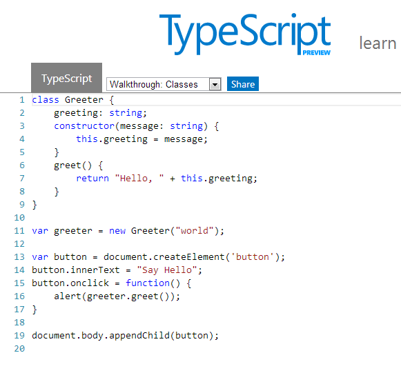
There is a live playground available for online experimentation with a few samples at disposal: http://www.typescriptlang.org/Playground/

Things I liked in Typescript

Static value declaration

As i said earlier declaring a variable in JS is simply assigning a value to it, the rest of internal operations are up to the JIT compiler. This is the root of many unwanted errors which happens when we unconsciously  messing up different types of values with the originally declared variable. Typescript helps to resolve this issue by allowing to statically declare the variable type. If no type has been specified the type any is inferred.

var num: number = 20;

which compiles to JS as:

var num = 20;

The only chance in JS to get feedback about the errors is to use test cases by covering all the possible errors you might expect:

if typeof num !== "number" {
   throw new Error(num, " is not a number");
}

On the other hand TS informs instantly about the errors as you type.

Arrow function expression

Another great feature is the addition of the so called arrow function expression. These are useful on situations when we need to preserve the scope of the outer execution context. A common practice widespread among JS developers is to bind this to a variable self which we place outside the inner function.
A function expression using the function keyword introduces a new dynamically bound this, whereas an arrow function expression preserves the this of its enclosing context. These are particularly useful in situation when we need to write callbacks like in the following example.

function sayHello(message:string, callback:()=>any) {
	alert(message);
	setTimeout(callback, 2000);
}

sayHello("Welcome visitor", function() {
	alert("thank you");	
});

Classes, modules, interfaces

Probably the greatest addition of Typescript is the possibility to work with classes, modules and interfaces.

Interfaces

Let’s start with interfaces. In Typescript interfaces have only a contextual scope, they haven’t any runtime representations of the compiled code. Their role is only to create a syntactic structure, a shell which is particular useful for object properties validation, in other words for documenting and validating the required shape of properties, objects passed as parameters, and objects returned from functions. In TS, interfaces are actually object types. While in Actionscript you have to have a class to implement the interface, in TS a simple object can implement it. Here is how you declare interfaces in TS:

interface Person {
	name: string;
	age?: number;
}

function print(person: Person) {
	if (person.age) {
		alert("Welcome " + person.name + " you are " + person.age + " age");	
	} else {
		alert("Welcome " + person.name);
	}
	
}

print({name: "George", age:22});

Furthermore interfaces have function overloading features which means that you can pass two identical functions on the same interface and let the user decide at the implementation phase which function wants to implement:

interface Overload {
	foo(s:string): string;
	foo(n:number): number;
}

function process(o:Overload) {
	o.foo("string");
	o.foo(23);
}

Another very interesting particularity of Typescript is that above the support offered for overloading functions, this is applicable for constructors too. This way we can redefine multiple constructor only by changing the way we implement it.

var canvas = document.createElement("canvas");
document.body.appendChild(canvas);
var ctx = canvas.getContext('2d');

interface ICircle {
	x: number;
	y: number;
	radius: number;
	color?: string;
}

class Circle {
	public x: number;
	public y: number;
	public radius: number;
	public color: string = "#000";
	
	constructor () {}		
	
	constructor () { 
		this.x = Math.random() * canvas.width;
		this.y = Math.random() * canvas.height;
		this.radius = 40;
	}		 		
	
	constructor (circle: ICircle = {x:Math.random() * canvas.width, y:Math.random() * canvas.height, radius:20}) {
		this.x = circle.x;
		this.y = circle.y;
		this.radius = circle.radius;
	}
}

var c = new Circle();
ctx.fillStyle = c.color;
ctx.beginPath();
ctx.arc(c.x, c.y, c.radius, 0, Math.PI * 2, true);
ctx.closePath();
ctx.fill();

Classes

The most advanced feature of Typescript (from my point of view) is the addition of the more traditional class structure with all the hotness like inheritance, polymorphism, constructor functions etc. In Typescript we are declaring the class in the following way:

class Point {
	x: number;
	y: number;
	
	constructor(x: number, y: number) {
		this.x = x;
		this.y = y;
	}
	
	sqrt() {

		return Math.sqrt(this.x * this.x + this.y * this.y) 
	}
	
	print(callback?) {		 
		setTimeout(callback, 3000);
		
	}
}

class Point3D extends Point {	
	z : number;
	
	constructor ( x:number,  y: number, z: number) {
		super(x, y);
	}
	
	sqrt() {
		var d = super.sqrt();
		return Math.sqrt(d * d + this.z * this.z);
	}
}

var p = new Point(20, 20);
p.print(() => { alert (p.sqrt()); });

… which in Javascript compiles to:

var __extends = this.__extends || function (d, b) {
    function __() { this.constructor = d; }
    __.prototype = b.prototype;
    d.prototype = new __();
};
var Point = (function () {
    function Point(x, y) {
        this.x = x;
        this.y = y;
    }
    Point.prototype.sqrt = function () {
        return Math.sqrt(this.x * this.x + this.y * this.y);
    };
    Point.prototype.print = function (callback) {
        setTimeout(callback, 3000);
    };
    return Point;
})();
var Point3D = (function (_super) {
    __extends(Point3D, _super);
    function Point3D(x, y, z) {
        _super.call(this, x, y);
    }
    Point3D.prototype.sqrt = function () {
        var d = _super.prototype.sqrt.call(this);
        return Math.sqrt(d * d + this.z * this.z);
    };
    return Point3D;
})(Point);
var p = new Point(20, 20);
p.print(function () {
    alert(p.sqrt());
});

Analyzing the code we observe that it share almost the same principle like any other static type language. We declare the class, it’s variables and functions, which can be static, private and public. By default the declared functions and variables are public, but we can make them private or static, by placing the private or static keyword in front of them. TS supports the constructor functions, which we declare in the following format:

var1:type;
var2:type;
constructor (var1:type, var2:type...varn:type) {
       this.var1 = var1;
       this.var2 = var2;
       .
       .
       .
       this.varn = varn;
}

It’s possible to declare the constructor arguments type as public and then we can eliminate to assign the constructor function parameters to constructor’s variables.

Typescript facilitates the working with classes by introducing another two great features commonly used in OOP, namely the inheritance and class extension. I rewrite the above code sample to show with a few simple changes we can extend the existing code to embrace some advanced polymorphism methods:

class Point {
	x: number;
	y: number;
	
	constructor(x: number, y: number) {
		this.x = x;
		this.y = y;
	}
	
	sqrt(x:number, y:number):number {		
		return Math.sqrt(x * x + y * y); 
	}
	
	dist(p:Point):number {
		var dx: number = this.x - p.x;
		var dy: number = this.y - p.y;
		
		return this.sqrt(dx, dy);
	}
	
	print(callback?) {		 
		setTimeout(callback, 3000);
		
	}
}

class Point3D extends Point {	
	z : number;
	
	constructor ( x:number,  y: number, z: number) {
		super(x, y);
	}
	
	sqrt3(z:number) {
		var s = super.sqrt(this.x, this.y);
		return Math.sqrt(s * s + this.z * this.z);		
	}	
		
	dist(p:Point3D):number {
		var d = super.dist(p);		
		var dz: number = this.z - p.z;										
		return this.sqrt3(dz);
	}
}

var p = new Point3D(19, 20, 20);
p.print(() => { alert (p.dist(new Point3D(2,2,20))); });

Modules

The last topic i want to discuss is about modules. Typescript module implementation is closely aligned with ECMAScript 6 proposal and supports code generation, targeting AMD and CommonJS modules. There are two types of source files Typescript is supporting: implementation source files and declaration source files. The difference between the two is that the first one contains statements and declarations, on the other hand the second contains only declarations. These can be used to declare static type information associated with existing javascript code. By default, a JavaScript output file is generated for each implementation source file in a compilation, but no output is generated from declaration source files.

The scope of modules is to maintain a clean structure in our code and to prevent the global namespace pollution. If suppose i have to create a global function Main the way i do in Javascript without to override the function at a later stage is to assure that the Main function get initialized only once. This is a common technique widespread among JS developers. In TS we do in the following way:

module net.esimov.core {
	export class Main {
		public name: string;
		public interest: string;
		
		constructor() {
			this.name = "esimov";
			this.interest = "web technology";
		}
		
		puts() {
			console.log(this.name, " like", this.interest);
		}
	}
}

Importing the declaration files is simple as placing the following statement on the top of our code: /// <reference path="...";/>. Then with a simple import statement we’ll import the modules needed at one specific moment.

import Core = net.esimov.core;
var c = new Core.Main();

Final thoughts

Typescript is a language that is definitely worth to try it. Unfortunately it has one main disadvantage, namely to benefit from it’s strong typing features we need to declare and construct declaration files for libraries we want to include in our projects. There are predefined declaration files for jQuery, node.js and d3.js, just to mention a few, but hopefully as the community will grow this list will get bigger and bigger.

Another weak point is the lack of support from IDE’s other than MS Visual Studio, but fortunately Webstorm 6 has in perspective to include full type support for Typescript too.

What’s next?

With this introduction done, my intention is to put into real usage all the information and learning accumulated and trying to create some canvas experiments but this time using Typescript. So check out soon.

Other resources to check

• Codeplex – project hosting
• Typescript playground – Playground for online experimentation
• TypeScript for ActionScript Developers – back-to-back comparison with AS2/AS3
• Support for Typescript on Stackoverflow