Category: Generative

Coherent Line Drawing implementation in Go (GoCV)

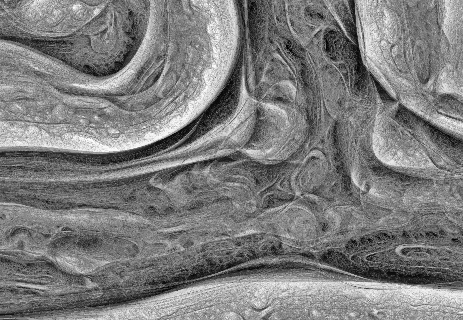
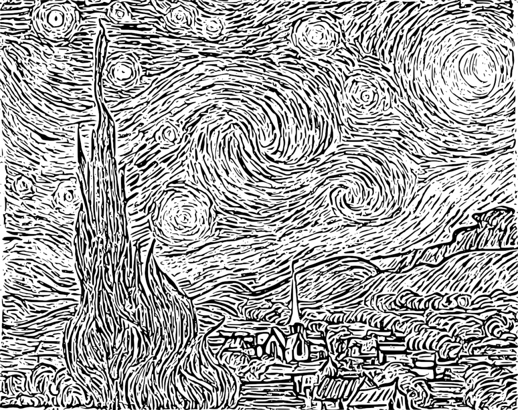
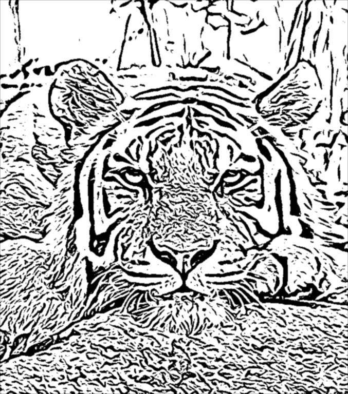
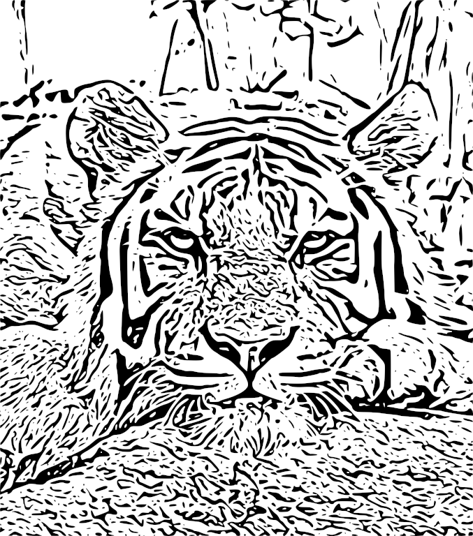
Surfing the web a beautiful, pencil-drawn like image captured my attention, it looked like as a hand-drawn image, but also became almost evident that it was a computer generated art. I found that it was created using an algorithm known as Coherent Line Drawing.

Introduction

In the last period of time I have been working on and off (as my limited free time permitted) on the implementation of the Coherent Line Drawing algorithm developed by Kang et al. Only now I considered that the implementation is so stable that I can publish it, so here it is: https://github.com/esimov/colidr.

Since my language of choice was Go I decided to give it a try implementing the original paper in Go, more explicitly in GoCV, an OpenCV wrapper for Go. I opted for this choice since the implementation is heavily based on linear algebra concepts and requires to work with matrices and vector spaces, things in what OpenCV notoriously excels.

However some of the functions required by the algorithm were missing from the GoCV codebase (at that period of time) like Sobel, uniformly-distributed random numbers and also vector operations like getting and setting the vector values. Meantime checking the latest release I found that the core codebase has been extended with some of the missing functionalities like the Sobel threshold, bitwise operations etc., however there were still missing pieces required by the algorithm. For this reason I have extended the GoCV code base with the missing OpenCV functionalities and included into the project as vendor dependency. Probably in the upcoming future I will create a pull request to merge it back in the main repository.

I won’t go into too much detail about the algorithm itself, you can find it in the original paper. I will discuss mostly about the technical difficulties encountered during the implementation, but also about the challenges imposed by gocv and OpenCV.

Why Go?

Now let’s talk about the challenges imposed by the project. The first question which might arise is why in Go, knowing that Go is not really appealing for creative coding, and it is mostly used in automatization, infrastructure, devops and web programming.

From my first acquaintance with Go (which was quite a few years back) I was intrigued by the potential possibilities offered by the language to make use of it in fields like image processing, computer vision, creative coding etc, since these are the fields i’m mostly interested in, and almost all of my open source project developed in Go have circulated around this topic. So this project was another attempt of mine to demonstrate that the language is well suited for these kind of projects too.

Go has a small package for image operations, but it is fair enough for anything you need to read an image file, obtain and manipulate the pixel values and finally to encode the result into an output file. Everything is concise and well structured. Since in this project we mostly rely on the OpenCV embedded functions provided by GoCV, there are still plenty of use cases when you need to rely on the core image library. Go does not provide a high level, abstract function to modify the source image, you need to access the raw pixel values in order to modify them.

Another key aspect in the language choice was that Go has an out of the box command line flag parsing library, just what I needed, since I conceived this application to be executed from the terminal. Maybe in the upcoming future I will create a GUI version too.

Technical challenges

Going back to the technical challenges I encountered during the implementation, one of the main headaches was related to how sensible OpenCV is to the way the types of matrices are declared. I was banging my head into the wall many times for the simple reason that my matrices were defined as gocv.MatTypeCV32F, however they should have been defined as gocv.MatTypeCV32F+gocv.MatChannels3, since the concatenation of these two variables were producing the desired matrix type value declared in the underlying OpenCV code base. More exactly by creating a new Mat and defining it’s type as simply MatTypeCV32F, the underlying gocv method will call the Mat_NewWithSize C method, having the last parameter the type of the matrix. Exactly this kind of limitation have confused me, ie. not all of the supported OpenCV mat types have been defined in the GoCV counterpart.

Since OpenCV is very flexible on matrix operations and won’t complain about the matrix conversions from one type to another, there are some edge cases when they are producing undesired results. This is a thing you have to consider when you are doing matrix operations in OpenCV: you need to be aware of the matrix type, otherwise your end results could be utterly compromised.

However comparing the OpenCV and GoCV matrix type tables, a lot of types are still missing from GoCV. For this simple “thing” my outputs were far from desirable from what it should have been. I was spinning in round and round, going back and forth, trying different solutions, comparing the code with the pseudo algorithms and formulas provided in the original paper to finally realizing that my matrices were defined with the wrong type or because some of the types declared in OpenCV were completely missing from the GoCV counterpart. The solution was either to extend the core code base or to concatenate the two matrix types (as presented above) in order to produce the correct type value requested by OpenCV.

Another elementary thing which is missing from GoCV is the SetVecAt method for setting or updating the vector values, even though a method for retrieving the vector values does exists. My initial attempt was to modify the vector values on byte level and encode it back into a matrix using the GoCV NewMatFromBytes method, which proved to be completely inefficient.

<br />

The solution was to extend the core GoCV codebase with a SetVec method.

<br />

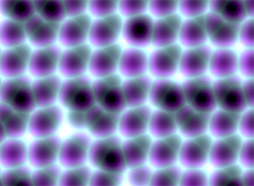
Another thing I learned is converting one matrix type to another does not always work as you think. I experienced this issue when during the debugging session I had to convert a float64 matrix to uint8, which can be exported as a byte array needed for the final binary encoding. It worked, but converting back to a float64 matrix requested by rotateFlow method didn’t not produced the desired output. (This method applies a rotation angle on the original gradient field and calculates the new angles.)

<br />

Since Go is using strict types for variable declarations, the auto casting is not possible like in C or C++. For this reason you need to pay attention to how you are converting the values from one type to another. Because GoCV / OpenCV matrices defined as floats are using 32 bits precision float values we need to be cautious when we have to cast a value defined as float64 for example to a 32 bit integer. This was the case on edge tangent flow visualization.

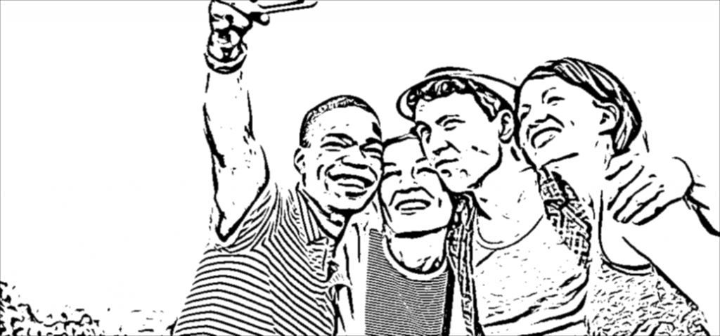
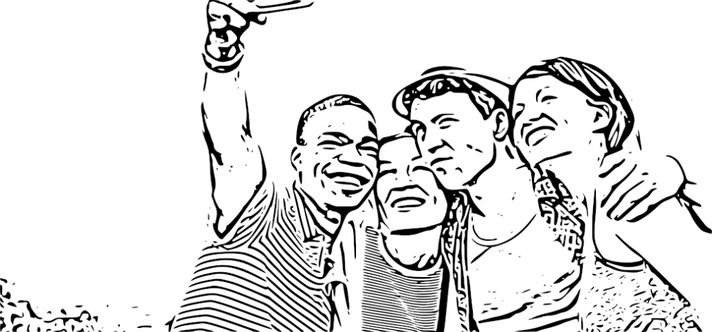
The examples below were produced with the wrong (left) and good type casting (right).

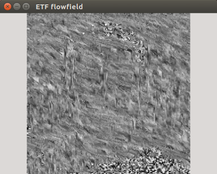
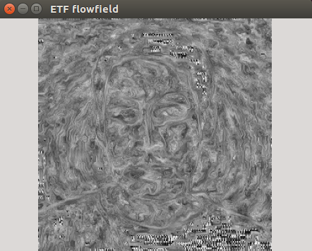
Even though the paper provided the implementation details for ETF visualization, my first attempt of it’s implementation didn’t produced the correct results. Only when I printed out the results I realized that the values were spanning over the range of the 32 bit integers, however OpenCV does not complained about this. The solution for this problem was to cast the index values of the for loop iterator as float32.

<br />

This is a takeaway you have to consider when you are working with OpenCV matrix types, especially in a language like Go, which is very strict in terms of variable types definition.

Conclusion

To sum up: GoCV is a welcome addition for the Go ecosystem, considering that it is under development many of the core OpenCV features are already implemented. However as I mentioned above there are still missing features, which should be addressed to become a viable OpenCV wrapper for the Go ecosystem. What I have learned using OpenCV is that you have to tinker with the values, and slight changes on the inputs can produce completely broken outputs, so you need to find that tiny middle road where the different equation parameters can converge.

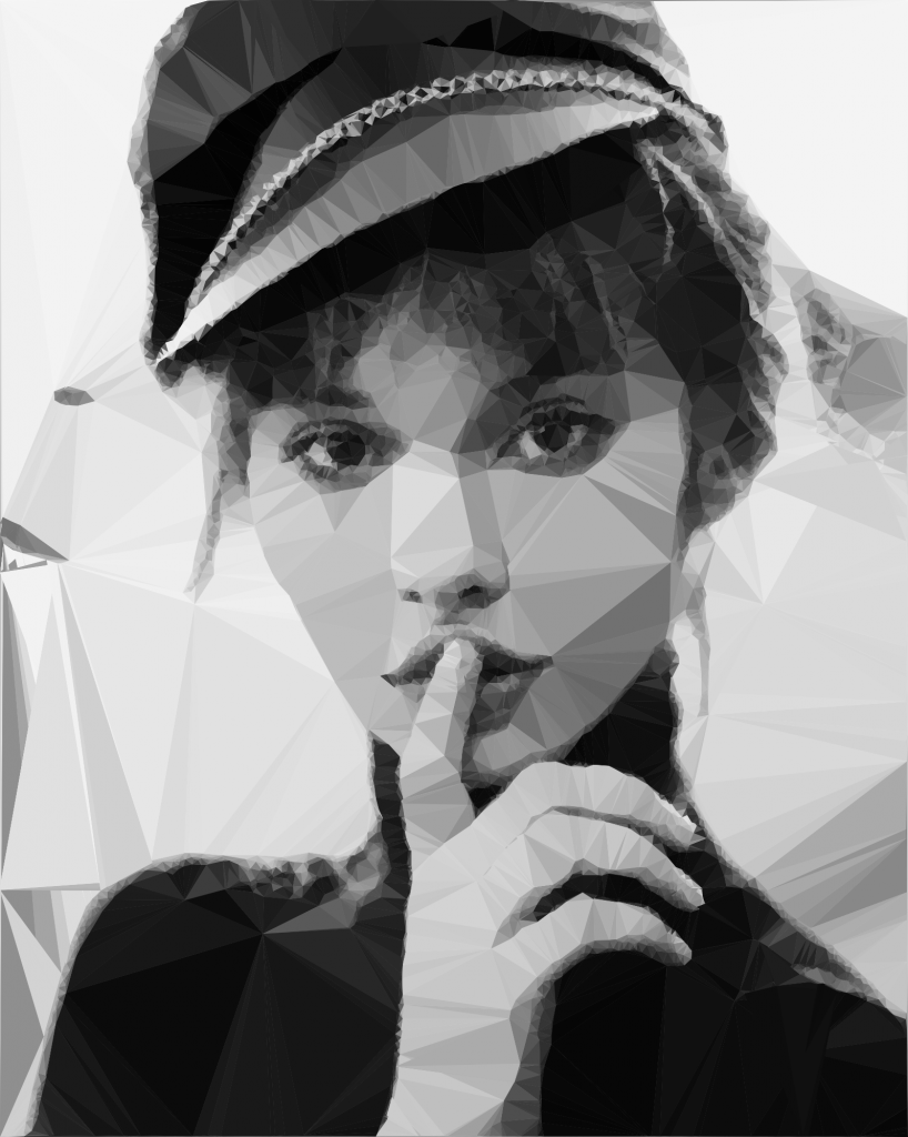
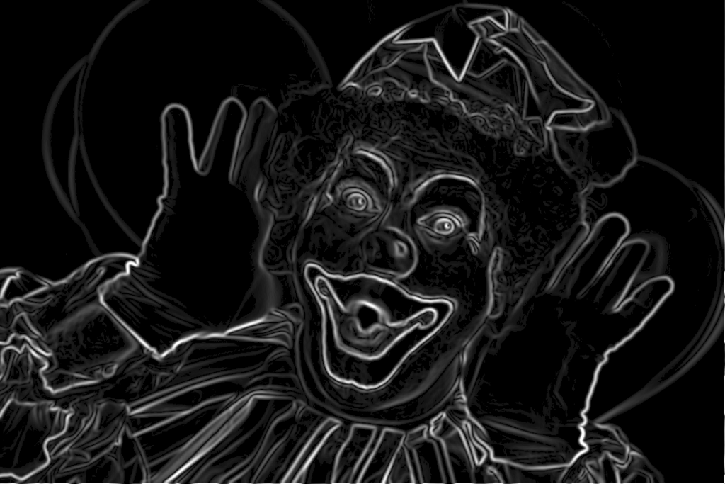
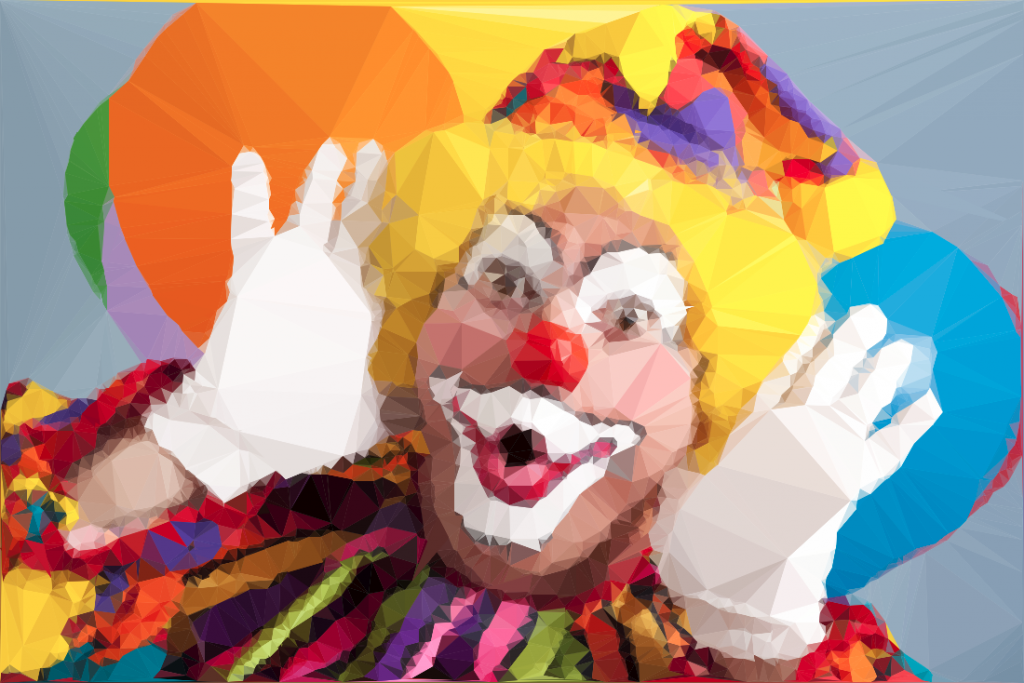
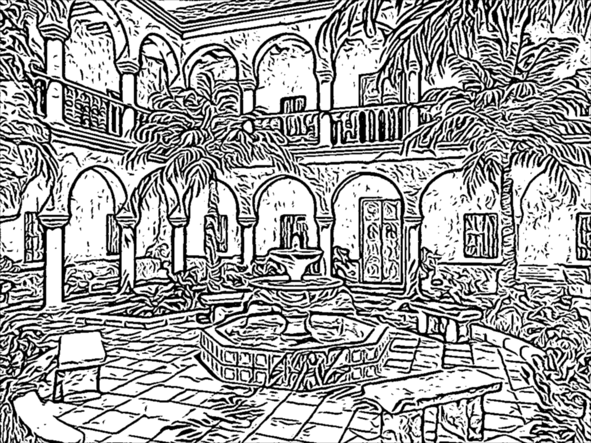
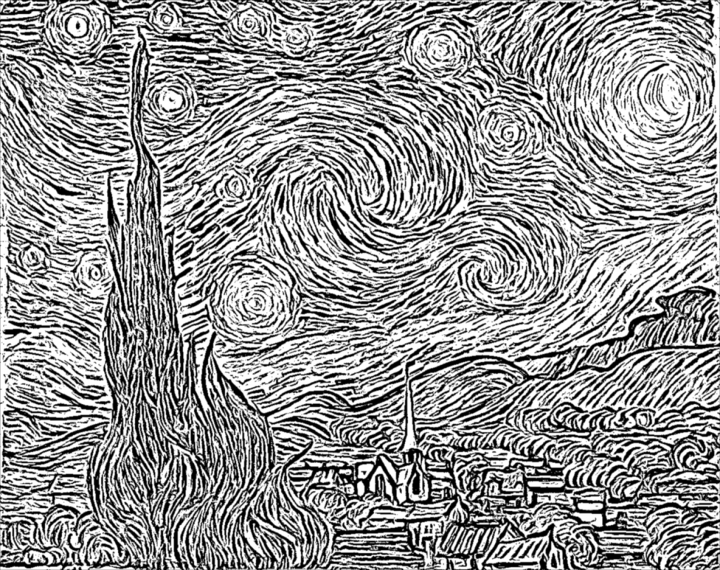
Sample images

Source code

The code is open source and can be found on my Github page:

https://github.com/esimov/colidr

You can follow me on twitter too: https://twitter.com/simo_endre

July 10, 2019
Delaunay image triangulation
In this article we present a technique to triangulate source images, converting them to abstract, someway artistic images composed of tiles of triangles. This will be an attempt to explore the fields between computer technology and art.

But first, what is triangulation? Simply spoken a triangulation partitions a polygon into triangles which allows, for instance, to compute the area of a polygon and execute some operations on the computed polygon surface. In other terms the triangulation might be conceived as a geometric object defined by a point set, but what differentiates the polygons from a point set is the latter does not have an interior, except if we treat the point set as a convex hull/polygon. But to think of a point set as a convex polygon, the points from the interior of the convex hull should not be ignored completely. This is what differentiates the Delaunay triangulation from the other triangulation techniques.

Fig.1: Point set triangulation.

Delaunay triangulation

Wikipedia has a very succinct definition of the Delaunay triangulation:

… a Delaunay triangulation (also known as a Delone triangulation) for a given set P of discrete points in a plane is a triangulation DT(P) such that no point in P is inside the circumcircle of any triangle in DT(P)

The circumcircle of a triangle is the unique circle passing through all the vertices of the triangle. This will get valuable meaning in the following. So considering that we have a set of six points we can obtain a triangulated polygon by tracing a circle around each vertex of the constructed triangle in such a manner that the circumcircle of all five triangles are empty. We also say, that the triangles satisfy the empty circle property (Fig.2).

Fig.2: All triangles satisfy the empty circle property.

After a short theoretical introduction now we want to apply this technique to a more practical but at the same time aesthetical field, concretely to transform a source image to it’s triangulated counterpart. Having the basic idea and it’s theoretical background we can start to construct the basic building blocks of the algorithm.

Above all a short notice: we use Go as programming language for the implementation. First, because it has a very clean and easy to use API, second because it can be well suited for a CLI based application, which single scope is to convert an input file to a destination object.

The algorithm

Now into the algorithm. As the basic components are triangles we define a Triangle structs, having as constituents the nodes, it’s edges and the circumcircle which describes the triangle circumference.
```
type Triangle struct {
      Nodes  []Node
      edges  []edge
      circle circle
}
```
Next we create the circumscribed circle of this triangle. The circumcircle of a triangle is the circle which has the three vertices of the triangle lying on its circumference. Once we have the circle center point we can calculate the distance between the node points and the triangle circumcircle. Then we can calculate the circle radius.

We can transpose this into the following Go code:

<br />

The question is how do we get the triangle points from the input image? To obtain a large triangle distribution on the image parts with more details we need somehow to analyze the image and mark the sensitive information. How do we do that? Sobel filter operator on the rescue. The Sobel operator is used in image processing to detect image edges. It’s working with an energy distribution matrix to differentiate the sensitive image informations from the less sensitive ones.

Fig.3: Sobel operator applied to the source image.

Once we obtained the sobel image we can sparse the triangle points randomly by applying some threshold value. At the end we obtain an array of randomly distributed points, but these points are more dense on the sensitive image parts, and scarce on less sensitive ones.

Having the edge points we check whether the points are inside the triangle circumcircle or not. We save the triangle edges in case they are included and carry over otherwise. Then in a loop we search for (almost) identical edges and remove them.

<br />

Now that we have the nodes, in order to construct the triangulated image, the last thing we need to do is actually to draw the lines between nodes points by applying the underlying image pixel colors. The way we can achieve this is to loop over all the nodes and connect each edge point.

<br />

By tweaking the parameters we can obtain different kind of results. We can draw only the line strokes, we can apply different threshold values to filter out some edges, we can scale up or down the triangle sizes by defining the maximum point limit, we can export only to grayscale mode etc. The possibilities are endless.

Fig.4: Triangulated image example.

Using Go interfaces to export the end result into different formats

By default the output is saved to an image file, but using interfaces, the Go way to achieve polymorphism, we can export even to a vector format. This is a nice touch considering that using a small image as input element we can export the result even to an svg file, which lately can be scaled up infinitely without image loss and consuming very low processing footprint.

The only thing we need to do is to declare an interface having a single method signature. This needs to be satisfied by each struct type implementing this method.

<br />

In our case we need two struct types, both of them implementing the same method differently. For example we could have an image struct type and an svg struct type declared in the following way:

<br />

Each of them will implement the same Draw method differently.

Expose the algorithm as an API endpoint

Having a good system architecture, coupled with Go blazing fast execution time and goroutines (another feature of the Go language to parallelize the execution) the algorithm can be exposed to an API endpoint in order to process a large amount of images and then make it accessible through a web application.

The source code can be found on my Github page:

https://github.com/esimov/triangle

I have also created an Electron/React desktop application for everyone who do not want to be bothered with the terminal commands and needs something more user friendly.

The source file can also be found on my Github account:
https://github.com/esimov/triangle-app
April 29, 2019
Navier Stokes Fluid Simulation on HTML5 Canvas
Implementing real time fluid simulation in pure Javascript was a long desire of me and has been sitting in my todo list from a long time on. However from various reasons i never found enough time to start working on it. I know it’s nothing new and there are quite a few implementations done on canvas already (maybe the best known is this: http://nerget.com/fluidSim/), but i wanted to do mine without to relay to others work and to use the core logic as found on the original paper.

For me one of the most inspiring real-time 2D fluid simulations based on Navier Stokes equations was that created by Memo Akten, originally implemented in Processing (a Java based programming language, very suitable for digital artists for visual experimentation), lately ported to OpenFrameworks (a C++ framework) then implemented in AS 3.0 by Eugene Zatepyakin http://blog.inspirit.ru/?p=248.

The code is based on Jos Stam’s famous paper – Real-Time Fluid Dynamics for Games, but another useful resource which i found during preparation and development was a paper from Mike Ash: Fluid Simulation for Dummies. As the title suggest, the concept is explained very clearly even if the equations behind are quite complex, which means without a good background in physics and differential equations it’s difficult to understand. This does not means that i’m a little genius in maths or physics :). In this post i will sketch briefly some of the main concepts behind the theory and more importantly how can be implemented in Javascript. As a side note, this simulation does not take advantages of the GPU power, so it’s not running on WebGL. For a WebGL implementation see http://www.ibiblio.org/e-notes/webgl/gpu/fluid.htm.

The basic concept

We can think of fluids as a collection of cells or boxes (in 3D), each one interacting with it’s neighbor. Each cell has some basic properties like velocity and density and the transformation taking place in one cell is affecting the properties of neighbor cells (all of these happening million times per second).

Being such a complex operation, computers (even the most powerful ones) can not simulate real time the fluid dynamics. For this we need to make some compromise. We’ll break the fluid up into a reasonable number of cells and try to do several interactions per second. That’s what Jos Stam’s approaching is doing great: sacrifice the fluid accuracy for a better visual presentation, more suitable for running real time. The best way to improve the simulation fluency is to reduce the solver iteration number. We’ll talk about this a little bit later.

First we are staring by initializing some basic properties like the number of cells, the length of the timestamp, the amount of diffusion and viscosity etc. Also we need a density array and a velocity array and for each of them we set up a temporary array to switch the values between the new and old ones. This way we can store the old values while computing the new ones. Once we are done with the iteration we need to reset all the values to the default ones. For efficiency purposes we’ll use single dimensional array over double ones.

The first step is to add some density to our cells:
```
function addDensitySource(x, x0) {                
	var size = self.numCells;        
	while(size-- > -1) {
		x[size] += _dt * x0[size];
	}
}
```
then to add some velocity:
```
FSolver.prototype.addCellVelocity = function() {
	var size = self.numCells;
	while(size-- > -1) {
		if (isNaN(self.u[size])) continue;
		self.u[size] += _dt * self.uOld[size];
		if (isNaN(self.v[size])) continue;
		self.v[size] += _dt * self.vOld[size];
	}
}
```
Because some of the functions needs to be accessible only from main script i separated the internal (private) functions from the external (public) functions. But because Javascript is a prototypical language i used the object prototype method to extend it. That’s why some of the methods are declared with prototype and others as simple functions. However these aren’t accessible from the outside of FS namespace, which is declared as a global namespace. For this technique please see this great article Learning JavaScript Design Patterns.

The process

The basic structure of our solver is as follows. We start with some initial state for the velocity and the density and then update its values according to events happening in the environment.
In our prototype we let the user apply forces and add density sources with the mouse (or we can extend this to touching devices too). There are many other possibilities this can be extended.

Basically to simulate the fluid dynamics we need to familiarize our self with three main operations:

Diffusion:

Diffusion is the process when – in our case – the liquids doesn’t stay still, but are spreading out. Through diffusion each cell exchanges density with its direct neighbors. The array for the density is filled in from the user’s mouse movement. The cell’s density will decrease by losing density to its neighbors, but will also increase due to densities flowing in from the neighbors.

Projection:

This means the amount of fluid going in has to be exactly equal with the amount of fluid going out, otherwise may happens that the net inflow in some cells to be higher or lower than the net inflow of the neighbor cells. This may cause the simulation to react completely chaotic. This operation runs through all the cells and fixes them up to maintain in equilibrium.

Advection:

The key idea behind advection is that moving densities would be easy to solve if the density were modeled as a set of particles. In this case we would simply have to trace the particles though the velocity field. For example, we could pretend that each grid cell’s center is a particle and trace it through the velocity field. So advection in fact is a velocity applied to each grid cell. This is what makes things move.

setBoundary():

We assume that the fluid is contained in a box with solid walls: no flow should exit the walls. This simply means that the horizontal component of the velocity should be zero on the vertical walls, while the vertical component of the velocity should be zero on the horizontal walls. So in fact every velocity in the layer next to the outer layer is mirrored. The following code checks the boundaries of fluid cells.
```
function setBoundary(bound, x) {
	var dst1, dst2, src1, src2, i;
	var step = FLUID_IX(0, 1) - FLUID_IX(0, 0);
	dst1 = FLUID_IX(0, 1);
	src1 = FLUID_IX(1, 1);
	dst2 = FLUID_IX(_NX+1, 1);
	src2 = FLUID_IX(_NX, 1);

	if (wrap_x) {
		src1 ^= src2;
		src2 ^= src1;
		src1 ^= src2;
	}

	if (bound == 1 && !wrap_x) {
		for (i = _NY; i > 0; --i) {
			x[dst1] = -x[src1]; dst1 += step; src1 += step;
			x[dst2] = -x[src2]; dst2 += step; src2 += step;
		}
	} else {
		for (i = _NY; i > 0; --i) {
			x[dst1] = x[src1]; dst1 += step; src1 += step;
			x[dst2] = x[src2]; dst2 += step; src2 += step;
		}
	}

	dst1 = FLUID_IX(1, 0);
	src1 = FLUID_IX(1, 1);
	dst2 = FLUID_IX(1, _NY+1);
	src2 = FLUID_IX(1, _NY);

	if (wrap_y) {
		src1 ^= src2;
		src2 ^= src1;
		src1 ^= src2;
	}

	if (bound == 2 && !wrap_y) {
		for (i = _NX; i > 0 ; --i) {
			x[dst1++] = -x[src1++];
			x[dst2++] = -x[src2++];
		}
	} else {
		for (i = _NX; i > 0; --i) {
			x[dst1++] = x[src1++];
			x[dst2++] = x[src2++];
		}
	}

	x[FLUID_IX(0, 0)] = .5 * (x[FLUID_IX(1, 0)] + x[FLUID_IX(0, 1)]);
	x[FLUID_IX(0, _NY+1)] = .5 * (x[FLUID_IX(1, _NY+1)] + x[FLUID_IX(0, _NY)]);
	x[FLUID_IX(_NX+1, 0)] = .5 * (x[FLUID_IX(_NX, 0)] + x[FLUID_IX(_NX+1, _NX)]);
	x[FLUID_IX(_NX+1, _NY+1)] = .5 * (x[FLUID_IX(_NX, _NY+1)] + x[FLUID_IX(_NX+1, _NY)]);
}
```
The main simulation function is implemented as follow:
```
FSolver.prototype.updateDensity = function() {        
	addDensitySource(this.density, this.densityOld);

	if (_doVorticityConfinement) {            
		calcVorticityConfinement(this.uOld, this.vOld);            
	}

	diffuse(0, this.densityOld, this.density, 0);
	advect(0, this.density, this.densityOld, this.u, this.v);
}

FSolver.prototype.updateVelocity = function() {
	this.addCellVelocity();
	this.SWAP('uOld', 'u');
	diffuse(1, this.u, this.uOld, _visc);
	this.SWAP('vOld', 'v');        
	diffuse(2, this.v, this.vOld, _visc);        
	project(this.u, this.v, this.uOld, this.vOld);

	this.SWAP('uOld', 'u');
	this.SWAP('vOld', 'v');
	advect(1, this.u, this.uOld, this.uOld, this.vOld);
	advect(2, this.v, this.vOld, this.uOld, this.vOld);
	project(this.u, this.v, this.uOld, this.vOld);
}
```
We are calling these functions on each frame on the main drawing method. For rendering the cells i used canvas putImageData() method which accepts as parameter an image data, whose values are in fact the fluid solver values obtained from the density array. My first attempt was to generate a particle field, associate to each particle density, velocity etc. (so all the data necessarily making a fluid simulation), connect each particle in a single linked list, knowing this is a much faster method for constructing an array, instead using the traditional one. Then using a fast and efficient method to trace a line, best known as Extremely Fast Line Algorithm or Xiaolin Wu’s line algorithm with anti aliasing (http://www.bytearray.org/?p=67) i thought i could gain more FPS for a smoother animation, but turned out being a very buggy implementation, so for the moment i abandoned the idea, but i will revised once i will have more time. Anyway i don’t swipe out this code part. You can find some utility functions too for my attempting, like implementing the AS3 Bitmap and BitmapData classes.

And here is the monochrome version:
www.esimov.com/experiments/javascript/fluid-solver-mono/

The simulation is fully adapted to touch devices, but i think you need a really powerful device to run the fluid simulation decently.

What’s next?

That’s all. Hopefully this will be a solid base to explore further this field and add some extra functionality.
January 6, 2014
Worley noise cellular texturing

There are some quite well known procedural content generation algorithms out there: Voronoi, Perlin noise, simplex noise, L-systems, reaction-diffusion systems like Turing pattern, which I’ve presented in my earlier blog post.The specifics of these algorithms are that either generates a large amount of content for a small investment of input data, or one that adds structure to random noise.

Generally speaking they are categorized by what they generate (map vs sequence generation) and also by the mindset behind their use. This time we’ll discuss the Worley noise pattern, which can be included into the generative map creation category. This means we need a grid system for the representation and visualization of points scattered randomly in 3D or 2D space.

In it’s visual appearance is almost like a Voronoi diagram, only it’s not as famous like it’s counterpart. Even Wikipedia discuss it very briefly. Worley noise in it’s essence is a noise generation pattern, which means by multiplication/addition of different octaves of the same noise pattern we can produce a variety and completely different outputs. This is the fun part of working with generative patterns.

Now, after we gain a little theoretical introduction let’s get started with the basics, and try to dissect how can we reproduce those organic shapes and textures found in every living being in nature. (In parentheses being said, in many graphic simulations and parametric applications dealing with textural visualizations this shapes can be found). As a last side note before we go into the technical details, my intention was to implement the algorithm in Javascript mainly because i wished to be accessible by as many users as possible, and at the same time i was curious how far can i stress the limit of the modern web browsers. This is an experiment based 100% on CPU, so WebGL was out of scope, only because i was not playing with this technology until now, but i considering to implement on GPU in a shorter or longer future.

Feature points

The basic idea is to spread randomly varying number in space and calculate the distance to these point from every possible location of space. As a complement, Worley suggest to assign to each feature point an unique ID number. This number can be used to generate surface with colored areas or crocodile like textures, cityblock diagrams etc. depending on the algorithm, or coloring function implemented.

The noise function simply computes a single value for every location in space. We can then use that value in literally thousands of interesting ways, such as perturbing an existing pattern spatially, mapping directly to a density or color or adding multiple scale of noise to make a fractal combination. While there are infinite number of possible functions which provide an infinite number of outputs, noise’s random behavior gives a much more interesting appearance then simple gradients for example.

By spreading feature points randomly through the 3D space we build a scalar function based on the distribution of the points near the sample location. Because an image worth a thousand of words the picture below describes a space with feature points scattered across the plane.

For a position on the plane (marked with x in the picture above) there is always a closest feature point, a second closest, a third and so on. The algorithm is searching for such feature points, return their relative distance to the target point, their position and their unique ID number.

Another key component of the algorithm is the demarcation line which is supposed to be integer in every plane. Each squares (cubes in 3D) are positioned so that their identification numbers can be expressed with some integer values. Let’s suppose we want to obtain the distance to the two feature point closest to the (3.6, 5.7) we start by looking at the integer squares (3, 5) and compare it’s feature points to each other. It’s obvius that the two feature points in that square aren’t the two closest. One of them is, but the second closest belongs to the integer square (3, 6).

It’s possible that some feature points are not inside the square where the target point is placed, in this case we extend our analysis to the adjacent squares. We could just test all 26 immediate neighboring cubes, but by checking the closest distance we’ve computed so far (our tentative n-th closest feature distance) we can throw out whole rows of cubes at once by deciding when no point in the neighbor cube could possibly contribute to our list. We don’t know yet what points are in the adjacent cubes marked by “?,” but if we examine a circle of radius F1, we can see that it’s possible that the cubes labeled A, B, and C might contribute a closer feature point, so we have to check them. As resulted from the image below, it’s mostly possible to check 6 facing neighbors of center cube (these are the closest and most likely to have a close feature point), 12 edge cube and 8 corner cubes in 3D. We could start testing more distant cubes, but it’s much more convenient to just use a high enough density to ensure that the central 27 are sufficient.

The code implementation in Javascript

For the code implementation i used html5 canvas. I’ve commented the source code, so won’t be too hard to follow for anyone. Because (as i mentioned in the beginning) my WebGL knowledge is quite minimal, for this reason i tried to optimize every single bit of code. For this reason my single option was to use web workers by separating the main core from the computationally heavy and intense pixel manipulation logic. There is a well described article on html5rocks.com about the basic principles of web workers, followed by some very neat examples regarding the implementation of them.

The main advantage of using web workers is that we can eliminate the bottlenecks caused by computational heavy threads running in the background, separating the implementation interface from the computational logic. This way we can reduce the hangouts caused by intensive calculations which may block the UI or script to handle the user interaction.

Creating a web worker is quite simple. We define the variables we want to pass to workers, and by calling an event listener using postMessage function we transfer the main tread instructions to the worker (which is running in a separate thread). Because web workers run in isolated threads, the code that they execute needs to be contained in a separate file. But before we do that, the first thing we have to do is create a new Worker object in our main page. The constructor takes the name of the worker script:

<br />

In a separate script we’ll define wich are the variables we want to listen for. This part is responsible for the heavy weight operations. After the pixel calculations has been done, we pass over the results through the postMessage method to the main thread. This part of code looks like the following:

<br />

As a last option i’ve included the DAT.GUI lightweight graphical interface for a user interaction, where we can select different methods, colors etc. and lastly to offer the possibility for rendering with or without web workers.

Hopefully you find interesting this experiment, and if you have some remarks, comments, then please use the comments field below, or share through twitter.

May 18, 2012
Organic Turing Pattern
In this post i will present an experiment which i did a few months earlier, but because lately i was pretty occupied with various job related activities and with setting up this new blog (transferring the old content to the new host – plus a lot of other stuff), i have no time to publish this new experiment. More about below, but until then a few words about the background, inspiration and some of the key challenge i have faced during this process.

This is an experiment inspired by a thoroughly explained article about the concept behind what is generally known as Turing Pattern. The Turing Patterns has become a key attraction in fact thanks to Jonathan McCabe popular paper Cyclic Symmetric Mutli-Scale Turing Patterns in which he explains the process behind the image generation algorithm like that one below, about what Frederik Vanhoutte know as W:blut wrote on his post:

If you’ve seen any reality zoo/wild-life program you’ll recognize this. Five minutes into the show you’re confronted with a wounded, magnificent animal, held in captivity so its caretakers can nurture and feed it. And inevitably, after three commercial breaks, they release it, teary-eyed, back into the wild. It’s a pivotal moment that turns their leopard into anyone’s/no one’s leopard.

That’s the feeling which emanates when you first see the organic like, somehow obscure (some may go even further and say: macabre or creepy) thing which is known as a Turing pattern. At first moment when you are confronted with it, some kind of emotion (be that fear or amazement or just a sight) is resurfaced. Definitely won’t let you neutral.

This is the emotion which pushed me to try to implement it in Actionscript. (In parentheses be said this is not the best platform for computation intensive experiments.) Felix Woitzel did an amazing ~~remake~~ adaptation of the original pattern in WebGL. The performance with a good GPU is quite impressive. Maybe in the future i will try to port in WebGL. Anyway, there is another nice article by Jason Rampe, where he explains the algorithm of the Turing Pattern.

So let’s face directly and dissect the core components of the algorithm.

The basic concept

The process is based on a series of different “turing” scales. Each scale has different values for activator, inhibitor, radius, amount and levels. We use a two dimensional grid which will be the basic container for activator, inhibitor and variations, all of them going to be of typed arrays (in our case Vectors.<>). At the first phase we will initialize the grid with random points between -1 and 1. In the next step we have to determine the shape of the pattern. For this case w’ll use a formula defined by the following method:
```
for (var i:int = 0; i < levels; i++)
{
	var radius:int = int(Math.pow(base, i));
	_radii[i] = radius;
	_stepSizes[i] = Math.log(radius) * stepScale + stepOffset;
}
```
During each step of simulation we have to execute the following methods:
1. Populate the grid with pixels at random locations. I’m gonna use a linked list to store the pixels properties: positions and colors. We will loop through all the pixels, the number of pixels will be defined by the grid with x height dimension.
2. Average each grid cell location over a circular radius specified by activator, then store the results in the activator array, multiplied by the weight.
3. Average each grid cell location over a circular radius specified by inhibitor, then store the results in the activator array, multiplied by the weight.
4. In the next step we need to calculate the absolute difference between the activator and inhibitor using the the following formula: variations = variations + abs(activator[x,y] - inhibitor[x,y])
Once we have all the activator, inhibitor and variations values calculated for each grid cells we proceed with updating the grids as follows:
1. Find which grid cell has the lowest variation value
2. Once we found the lowest variation value we update the grid by the following formula:
```
for (var l:Number = 0; l < levels - 1; l++)
{
	var radius:int = int(_radii[l]);
	fastBlur(activator, inhibitor, _blurBuffer, WIDTH, HEIGHT, radius);

	//calculates the absolute difference between activator and inhibitor

	for (var i:int = 0; i < n; i++)
	{
		_variations[i] = activator[i] - inhibitor[i];
		if (_variations[i] < 0)
		{
			_variations[i] = -_variations[i];
		}
	}

	//if first level then set some initial values for bestLevel and bestVariation 
	if (l == 0)
	{
		for (i = 0; i < n; i++)
		{
			_bestVariation[i] = _variations[i];
			_bestLevel[i] = l;
			_directions[i] = activator[i] > inhibitor[i];
		}
		activator = _diffRight;
		inhibitor = _diffLeft;
	}
	else
	{
		for (i = 0; i < n; i++)
		{
			if (_variations[i] < _bestVariation[i])
			{
				_bestVariation[i] = _variations[i];
				_bestLevel[i] = l;
				_directions[i] = activator[i] > inhibitor[i];

			}
		}
		var swap:Vector. = activator;
		activator = inhibitor;
		inhibitor = swap;
	}
}
```
As a last step we should average the gap between the levels by performing a blur technique for a nicer transition. We blur the image sequentially in two steps: first we blur the image vertically then horizontally.

The challenge

The most challenging part was related to the unknown factor about how well gonna handle the AVM2 the intensive CPU calculation. Well as you may have guessed not too well, especially with very large bitmap dimension and a lot of pixels needed to be manipulated, plus the extra performance loss “gained” after the bluring operation.

For some kind of compensation benefits (in terms of performance) i decided to populate the BitmapData with a chained loop using single linked list, plus typed arrays as generally known the Vector.<> arrays are much faster compared to the traditional array stacks. After a not too impressive performance, i wondered how can i even more optimize the code for a better overcome. I decided to give it a try to Alchemy, and Joa Ebert’s TDSI, a Java based Actionscript compiler, as by that time was commonly known a better choice over AVM. Unfortunately i didn’t get too many support and helpful articles about the implementation and as a consequence my attempt was a failure, which resulted in a quite buggy and ugly output. After too many attempts without the wishful result, i gave up.

That’s all in big steps. You can grab the source code from here. Feel free to post your remarks.

ps: Be prepared this experiment will burn your CPU. 🙂
February 25, 2012